Overview

Today, we dive deep into data analysis for causal inference ast it applies to observational cultural psychology. By the end, you will:

Better understand how to integrate measurement theory with causal inference
Enhance your proficiency in causal analysis using doubly robust methods
Gain insights into the application of sensitivity analysis using E-Values

Set up your workspace Preparing for the Journey

To kick things off, we will set up our environment. We’ll source essential functions, load necessary libraries, and import synthetic data for our exploration.

Code

# Before running this source code, make sure to update to the current version of R, and to update all existing packages.

# functions
source("https://raw.githubusercontent.com/go-bayes/templates/main/functions/funs.R")


# experimental functions (more functions)
source(
  "https://raw.githubusercontent.com/go-bayes/templates/main/functions/experimental_funs.R"
)


#  If you haven't already, you should have created a folder called "data", in your Rstudio project. If not, download this file, add it to your the folder called "data" in your Rstudio project. # "https://www.dropbox.com/s/vwqijg4ha17hbs1/nzavs_dat_synth_t10_t12?dl=0"

# A function we will use for our tables.
tab_ate_subgroup_rd <- function(x,
                                new_name,
                                delta = 1,
                                sd = 1) {
  # Check if required packages are installed
  required_packages <- c("EValue", "dplyr")
  new_packages <-
    required_packages[!(required_packages %in% installed.packages()[, "Package"])]
  if (length(new_packages))
    stop("Missing packages: ", paste(new_packages, collapse = ", "))
  
  require(EValue)
  require(dplyr)
  
  # check if input data is a dataframe
  if (!is.data.frame(x))
    stop("Input x must be a dataframe")
  
  # Check if required columns are in the dataframe
  required_cols <- c("estimate", "lower_ci", "upper_ci")
  missing_cols <- required_cols[!(required_cols %in% colnames(x))]
  if (length(missing_cols) > 0)
    stop("Missing columns in dataframe: ",
         paste(missing_cols, collapse = ", "))
  
  # Check if lower_ci and upper_ci do not contain NA values
  if (any(is.na(x$lower_ci), is.na(x$upper_ci)))
    stop("Columns 'lower_ci' and 'upper_ci' should not contain NA values")
  
  x <- x %>%
    dplyr::mutate(across(where(is.numeric), round, digits = 3)) %>%
    dplyr::rename("E[Y(1)]-E[Y(0)]" = estimate)
  
  x$standard_error <- abs(x$lower_ci - x$upper_ci) / 3.92
  
  evalues_list <- lapply(seq_len(nrow(x)), function(i) {
    row_evalue <- EValue::evalues.OLS(
      x[i, "E[Y(1)]-E[Y(0)]"],
      se = x[i, "standard_error"],
      sd = sd,
      delta = delta,
      true = 0
    )
    # If E_value is NA, set it to 1
    if (is.na(row_evalue[2, "lower"])) {
      row_evalue[2, "lower"] <- 1
    }
    if (is.na(row_evalue[2, "upper"])) {
      row_evalue[2, "upper"] <- 1
    }
    data.frame(round(as.data.frame(row_evalue)[2, ], 3)) # exclude the NA column
  })
  
  evalues_df <- do.call(rbind, evalues_list)
  colnames(evalues_df) <- c("E_Value", "E_Val_bound")
  
  tab_p <- cbind(x, evalues_df)
  
  tab <-
    tab_p |> select(c(
      "E[Y(1)]-E[Y(0)]",
      "lower_ci",
      "upper_ci",
      "E_Value",
      "E_Val_bound"
    ))
  
  return(tab)
}

# extra packages we need
# for efa/cfa
if (!require(psych)) {
  install.packages("psych")
  library("psych")
}

# for reporting
if (!require(parameters)) {
  install.packages("parameters")
  library("parameters")
}

# for graphing
if (!require(see)) {
  install.packages("see")
  library("see")
}

# for graphing
if (!require(lavaan)) {
  install.packages("lavaan")
  library("lavaan")
}


# for graphing
if (!require(datawizard)) {
  install.packages("datawizard")
  library("datawizard")
}

Import the data

# This will read the synthetic data into Rstudio.  Note that the arrow package allows us to have lower memory demands in the storage and retrieval of data.

nzavs_synth <- arrow::read_parquet(here::here("data", "nzavs_dat_synth_t10_t12"))

Next, we will inspect column names.

Make sure to familiarise your self with the variable names here

It is alwasy a good idea to plot the data (do on your own time.)

Revisit the checklist

As we delve deeper, it’s essential to remember our checklist:

Clearly state your question.
Explain its relevance.
Ensure your question is causal.
Develop a subgroup analysis question if applicable.

Our discussion today revolves around two main questions:

Does exercise influence anxiety/depression?
Do these effects differ among NZ Europeans and Māori?

While these questions offer a starting point, they lack specificity. We need to clarify:

The amount, regularity, and duration of exercise
The measures of depression to be used
The expected timeline for observing the effects

Remember, we can clarify these by emulating a hypothetical experiment, a concept we call the Target Trial.

This analysis has practical motivation, as the effects of exercise on mental health and possible differences between cultural groups remain largely uncharted territory.

Our initial responses will be guided by the NZAVS measure of exercise, focusing on the hours of activity per week, the 1-year effect on Kessler-6 depression after initiating a change in exercise, and a particular emphasis on effect-modification by NZ European and Māori ethnic identification. This analysis has practical motivation, as the effects of exercise on mental health and possible differences between cultural groups remain largely uncharted territory.

Sculpting the Data: A Hands-On Approach

As we venture further, we’ll perform a series of transformations to shape our data according to our needs. Our process will involve:

Constructing a Kessler 6 average score
Building a Kessler 6 sum score
Coarsening the Exercise score

Consider the ambiguity in the NZAVS exercise question: “During the past week, list ‘Hours spent exercising/physical activity’.” Different people interpret physical activity differently; John may consider any wakeful time as physical activity, while Jane counts only aerobic exercise. Such variation underlines the importance of the consistency assumption in causal inference. But we’ll delve deeper into that later.

For now, let’s transform our indicators.

# create sum score of kessler 6
dt_start <- nzavs_synth %>%
  arrange(id, wave) %>%
  rowwise() %>%
  mutate(lifesat_composite  = mean(
    c(lifesat_satlife,                         
    lifesat_ideal) ))|> 
  mutate(kessler_6  = mean(
    # Specify the Kessler scale items
    c(
      kessler_depressed,
      # During the last 30 days, how often did you feel so depressed that nothing could cheer you up?
      kessler_hopeless,
      # During the last 30 days, how often did you feel hopeless?
      kessler_nervous,
      # During the last 30 days, how often did you feel nervous?
      kessler_effort,
      # During the last 30 days, how often did you feel that everything was an effort?
      kessler_restless,
      # During the last 30 days, how often did you feel restless or fidgety ?
      kessler_worthless  # During the last 30 days, how often did you feel worthless?
    )
  )) |>
  mutate(kessler_6_sum = round(sum(
    c (
      kessler_depressed,
      kessler_hopeless,
      kessler_nervous,
      kessler_effort,
      kessler_restless,
      kessler_worthless
    )
  ),
  digits = 0)) |>  ungroup() |>
  # Coarsen 'hours_exercise' into categories
  mutate(
    hours_exercise_coarsen = cut(
      hours_exercise,
      # Hours spent exercising/ physical activity
      breaks = c(-1, 3, 8, 200),
      labels = c("inactive",
                 "active",
                 "very_active"),
      # Define thresholds for categories
      levels = c("(-1,3]", "(3,8]", "(8,200]"),
      ordered = TRUE
    ))|>
  # Create a binary 'urban' variable based on the 'rural_gch2018' variable
  mutate(urban = factor(
    ifelse(
      rural_gch2018 == "medium_urban_accessibility" |
        # Define urban condition
        rural_gch2018 == "high_urban_accessibility",
      "urban",
      # Label 'urban' if condition is met
      "rural"  # Label 'rural' if condition is not met
    )
  ))

Why do we coarsen the exposure? Recall the consistency assumption of causal inference:

Consistency: Can I interpret what it means to intervene on the exposure? I should be able to.

What is th hypothetical experiment here for change in exercise?

Through data wrangling, we can answer our research questions more effectively by manipulating variables into more meaningful and digestible forms. We imagine an experiment in which people were within one band of the coarsened exercise band and we

These data checks will ensure the accuracy and reliability of our transformations, setting the foundation for solid data analysis.

Code

# do some checks
levels(dt_start$hours_exercise_coarsen)
table(dt_start$hours_exercise_coarsen)
max(dt_start$hours_exercise)
min(dt_start$hours_exercise)
# checks


# justification for transforming exercise" has a very long tail
hist(dt_start$hours_exercise, breaks = 1000)
# consider only those cases below < or = to 20
hist(subset(dt_start, hours_exercise <= 20)$hours_exercise)
hist(as.numeric(dt_start$hours_exercise_coarsen))

Create variables for the latent factors

Let’s next get the data into shape for analysis. Here we create a variable for the two factors (see Appendix)

# get two factors from data
dt_start2 <- dt_start |>
  arrange(id, wave) |>
  rowwise() |>
  mutate(
    kessler_latent_depression = mean(c(kessler_depressed, kessler_hopeless, kessler_effort), na.rm = TRUE),
    kessler_latent_anxiety  = mean(c(kessler_effort, kessler_nervous, kessler_restless), na.rm = TRUE)
  ) |>
  ungroup()

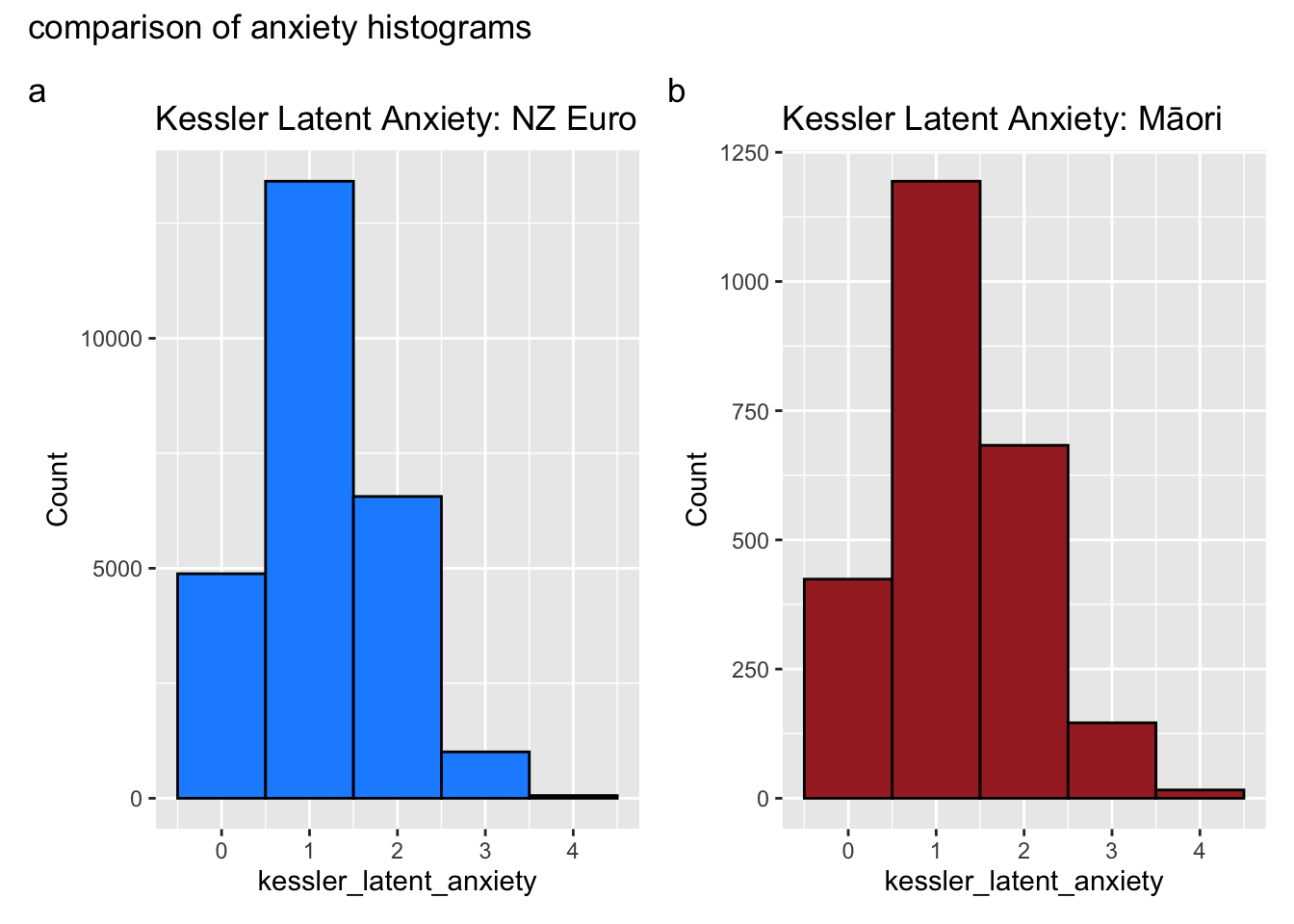
Inspect the data: anxiety

#hist(dt_start2$kessler_latent_anxiety, by = dt_start2$eth_cat)

create_histograms_anxiety <- function(df) {
  # require patchwork
  library(patchwork)
  
  # separate the data by eth_cat
  df1 <- df %>% filter(eth_cat == "euro") # replace "level_1" with actual level
  df2 <- df %>% filter(eth_cat == "māori") # replace "level_2" with actual level
  
  # create the histograms
  p1 <- ggplot(df1, aes(x=kessler_latent_anxiety)) +
    geom_histogram(binwidth = 1, fill = "dodgerblue", color = "black") +
    ggtitle("Kessler Latent Anxiety: NZ Euro") +
    xlab("kessler_latent_anxiety") +
    ylab("Count")
  
  p2 <- ggplot(df2, aes(x=kessler_latent_anxiety)) +
    geom_histogram(binwidth = 1, fill = "brown", color = "black") +
    ggtitle("Kessler Latent Anxiety: Māori") +
    xlab("kessler_latent_anxiety") +
    ylab("Count")
  
  # plot the histograms
 p1 + p2 + plot_annotation(tag_levels = "a", title = "comparison of anxiety histograms")
}

create_histograms_anxiety(dt_start2)

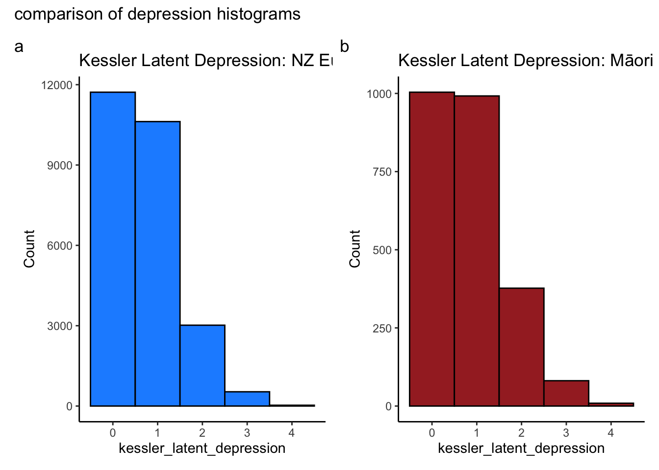
create_histograms_depression <- function(df) {
  # require patchwork
  library(patchwork)
  
  # separate the data by eth_cat
  df11 <- df %>% filter(eth_cat == "euro") # replace "level_1" with actual level
  df22 <- df %>% filter(eth_cat == "māori") # replace "level_2" with actual level
  
  # create the histograms
  p11 <- ggplot(df11, aes(x=kessler_latent_depression)) +
    geom_histogram(binwidth = 1, fill = "dodgerblue", color = "black") +
    ggtitle("Kessler Latent Depression: NZ Euro") +
    xlab("kessler_latent_depression") +
    ylab("Count") + theme_classic()
  
  p22 <- ggplot(df22, aes(x=kessler_latent_depression)) +
    geom_histogram(binwidth = 1, fill = "brown", color = "black") +
    ggtitle("Kessler Latent Depression: Māori") +
    xlab("kessler_latent_depression") +
    ylab("Count") + theme_classic()
  
  # plot the histograms
 p11 + p22 + plot_annotation(tag_levels = "a", title = "comparison of depression histograms")
}

create_histograms_depression(dt_start2)

What do you make of these histograms?

Investigate assumption of positivity:

Recall the positive assumption:

Positivity: Can we intervene on the exposure at all levels of the covariates? We should be able to.

Not this is just a description of the the summary scores. We do not assess change within indivuals

#  select only the baseline year and the exposure year.  That will give us change in the exposure. ()
dt_exposure <- dt_start2 |>

  # select baseline year and exposure year
  filter(wave == "2018" | wave == "2019") |>

  # select variables of interest
  select(id, wave, hours_exercise_coarsen,  eth_cat) |>

  # the categorical variable needs to be numeric for us to use msm package to investigate change
  mutate(hours_exercise_coarsen_n = as.numeric(hours_exercise_coarsen)) |>
  droplevels()


# check
dt_exposure |>
  tabyl(hours_exercise_coarsen_n, eth_cat,  wave )

$`2018`
 hours_exercise_coarsen_n euro māori pacific asian
                        1 3238   319      78   170
                        2 3790   341      81   130
                        3 1613   161      31    48

$`2019`
 hours_exercise_coarsen_n euro māori pacific asian
                        1 2880   307      79   143
                        2 3927   354      82   141
                        3 1834   160      29    64

I’ve written a function called transition_table that will help us assess change in the exposure at the individual level.

#   consider people going from active to vary active
out <- msm::statetable.msm(round(hours_exercise_coarsen_n, 0), id, data = dt_exposure)


# for a function I wrote to create state tables
state_names <- c("Inactive", "Somewhat Active", "Active", "Extremely Active")

# transition table

transition_table(out, state_names)

$explanation
[1] "This transition matrix describes the shifts from one state to another between the baseline wave and the following wave. The numbers in the cells represent the number of individuals who transitioned from one state (rows) to another (columns). For example, the cell in the first row and second column shows the number of individuals who transitioned from the first state (indicated by the left-most cell in the row) to the second state. The top left cell shows the number of individuals who remained in the first state."

$table


|      From       | Inactive | Somewhat Active | Active |
|:---------------:|:--------:|:---------------:|:------:|
|    Inactive     |   2186   |      1324       |  295   |
| Somewhat Active |   1019   |      2512       |  811   |
|     Active      |   204    |       668       |  981   |

Next consider Māori only

# Maori only

dt_exposure_maori <- dt_exposure |>
  filter(eth_cat == "māori")

out_m <- msm::statetable.msm(round(hours_exercise_coarsen_n, 0), id, data = dt_exposure_maori)

# with this little support we might consider parametric models
t_tab_m<- transition_table( out_m, state_names)

#interpretation
cat(t_tab_m$explanation)

This transition matrix describes the shifts from one state to another between the baseline wave and the following wave. The numbers in the cells represent the number of individuals who transitioned from one state (rows) to another (columns). For example, the cell in the first row and second column shows the number of individuals who transitioned from the first state (indicated by the left-most cell in the row) to the second state. The top left cell shows the number of individuals who remained in the first state.

print(t_tab_m$table)



|      From       | Inactive | Somewhat Active | Active |
|:---------------:|:--------:|:---------------:|:------:|
|    Inactive     |   187    |       108       |   24   |
| Somewhat Active |    92    |       188       |   61   |
|     Active      |    28    |       58        |   75   |

# filter euro
dt_exposure_euro <- dt_exposure |>
  filter(eth_cat == "euro")

# model change
out_e <- msm::statetable.msm(round(hours_exercise_coarsen_n, 0), id, data = dt_exposure_euro)


# creat transition table.
t_tab_e <- transition_table( out_e, state_names)

#interpretation
cat(t_tab_e$explanation)

This transition matrix describes the shifts from one state to another between the baseline wave and the following wave. The numbers in the cells represent the number of individuals who transitioned from one state (rows) to another (columns). For example, the cell in the first row and second column shows the number of individuals who transitioned from the first state (indicated by the left-most cell in the row) to the second state. The top left cell shows the number of individuals who remained in the first state.

# table
print(t_tab_e$table)



|      From       | Inactive | Somewhat Active | Active |
|:---------------:|:--------:|:---------------:|:------:|
|    Inactive     |   1843   |      1136       |  259   |
| Somewhat Active |   870    |      2208       |  712   |
|     Active      |   167    |       583       |  863   |

Overall we find evidence for change in the exposure variable. This suggest that we are ready to proceed with the next step of causal estimation.

Create wide data frame for analysis

Recall, I wrote a function for you that will put the data into temporal order such that measurement of the exposure and outcome appear at baseline, along with a rich set of baseline confounders, the exposure appears in the following wave, and the outcome appears in the wave following the exposure.

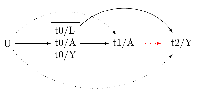
Figure 1: Causal graph: three-wave panel design

The graph encodes our assumptions about the world. It is a qualitative instrument to help us understand how to move from our assumptions to decisions about our analysis, in the first instance, the decision about whether to proceed with an analysis.

It is perhaps useful here to stop and consider what does this graph implies.

Question: 1. Does the graph imply unmeasured confounding?

Question 2. If there is unmeasured confounding, should we proceed?

E-value

The minimum strength of association on the risk ratio scale that an unmeasured confounder would need to have with both the exposure and the outcome, conditional on the measured covariates, to fully explain away a specific exposure-outcome association

See: [VanderWeele, Mathur, and Chen (2020)](Mathur et al. 2018)

For example, suppose that the lower bound of the the E-value was 1.3 with the lower bound of the confidence interval = 1.12, we might then write:

With an observed risk ratio of RR=1.3, an unmeasured confounder that was associated with both the outcome and the exposure by a risk ratio of 1.3-fold each (or 30%), above and beyond the measured confounders, could explain away the estimate, but weaker joint confounder associations could not; to move the confidence interval to include the null, an unmeasured confounder that was associated with the outcome and the exposure by a risk ratio of 1.12-fold (or 12%) each could do so, but weaker joint confounder associations could not.

The equations are as follows (for risk ratios)

E-value_{RR} = RR + \sqrt{RR \times (RR - 1)} E-value_{LCL} = LCL + \sqrt{LCL \times (LCL - 1)}

Here is an R function that will calculate E-values

calculate_e_value <- function(rr, lcl) {
  e_value_rr = rr + sqrt(rr*(rr - 1))
  e_value_lcl = lcl + sqrt(lcl*(lcl - 1))
  
  list(e_value_rr = e_value_rr, e_value_lcl = e_value_lcl)
}

# e.g. smoking causes cancer

# finding   RR = 10.73 (95% CI: 8.02, 14.36)

calculate_e_value(10.73, 8.02)

$e_value_rr
[1] 20.94777

$e_value_lcl
[1] 15.52336

We write:

With an observed risk ratio of RR=10.7, an unmeasured confounder that was associated with both the outcome and the exposure by a risk ratio of 20.9-fold each, above and beyond the measured confounders, could explain away the estimate, but weaker joint confounder associations could not; to move the confidence interval to include the null, an unmeasured confounder that was associated with the outcome and the exposure by a risk ratio of 15.5-fold each could do so, but weaker joint confounder associations could not.

Note that in this class, most of the outcomes will be (standardised) continuous outcomes. Here’s a function and LaTeX code to describe the approximation.

This function takes a linear regression coefficient estimate (est), its standard error (se), the standard deviation of the outcome (sd), a contrast of interest in the exposure (delta, which defaults to 1), and a “true” standardized mean difference (true, which defaults to 0). It calculates the odds ratio using the formula from Chinn (2000) and VanderWeele (2017), and then uses this to calculate the E-value.

#| label: evalue_ols

compute_evalue_ols <- function(est, se, delta = 1, true = 0) {
  # Rescale estimate and SE to reflect a contrast of size delta
  est <- est / delta
  se <- se / delta

  # Compute transformed odds ratio and confidence intervals
  odds_ratio <- exp(0.91 * est)
  lo <- exp(0.91 * est - 1.78 * se)
  hi <- exp(0.91 * est + 1.78 * se)

  # Compute E-Values based on the RR values
  evalue_point_estimate <- odds_ratio * sqrt(odds_ratio + 1)
  evalue_lower_ci <- lo * sqrt(lo + 1)

  # Return the E-values
  return(list(EValue_PointEstimate = evalue_point_estimate,
              EValue_LowerCI = evalue_lower_ci))
}




# exampl:
# suppose we have an estimate of 0.5, a standard error of 0.1, and a standard deviation of 1.
# This would correspond to a half a standard deviation increase in the outcome per unit increase in the exposure.
results <- compute_evalue_ols(est = 0.5, se = 0.1, delta = 1)
print(results)

$EValue_PointEstimate
[1] 2.529831

$EValue_LowerCI
[1] 2.008933

We write:

With an observed risk ratio of RR=2.92, an unmeasured confounder that was associated with both the outcome and the exposure by a risk ratio of 2.92-fold each, above and beyond the measured confounders, could explain away the estimate, but weaker joint confounder associations could not; to move the confidence interval to include the null, an unmeasured confounder that was associated with the outcome and the exposure by a risk ratio of 2.23-fold each could do so, but weaker joint confounder associations could not.

Note the E-values package will do the computational work for us (note we get slightly different estimates)

Note:

First, the fucntion converts the estimate to an odds ratio:

Odds Ratio Conversion:

(OddsRatio = e^{ })

Then, it calculates the confidence intervals for the odds ratio:

Confidence Intervals:

(LowerConfidenceInterval = e^{log(OddsRatio) - 1.78 SE})

(UpperConfidenceInterval = e^{log(OddsRatio) + 1.78 SE})

Finally, it calculates the E-value for the point estimate and the lower confidence interval:

E-Values Calculation:

(EValue_{PointEstimate} = OddsRatio + )

(EValue_{LowerCI} = LowerConfidenceInterval + )

[[JB: NEED TO CHECK]]

Generally, best to use the EValue function.

library(EValue)

EValue::evalues.OLS(est = 0.5, se = 0.1, sd = 1, delta = 1, true = 0)

            point    lower    upper
RR       1.576173 1.319166 1.883252
E-values 2.529142 1.968037       NA

############## ############## ############## ############## ############## ############## ############## ########
####  ####  ####  CREATE DATA FRAME FOR ANALYSIS ####  ####  ################## ############## ######## #########
############## ############## ############## ############## ############## ############## ############# #########


# I have created a function that will put the data into the correct shape. Here are the steps.

# Step 1: choose baseline variables (confounders).  here we select standard demographic variablees plus personality variables.

# Note again that the function will automatically include the baseline exposure and basline outcome in the baseline variable confounder set so you don't need to include these. 


# here are some plausible baseline confounders
baseline_vars = c(
  "edu",
  "male",
  "eth_cat",
  "employed",
  "gen_cohort",
  "nz_dep2018", # nz dep
  "nzsei13", # occupational prestige
  "partner",
  "parent",
  "pol_orient",
 # "rural_gch2018",
   "urban", # use the two level urban varaible. 
  "agreeableness",
  "conscientiousness",
  "extraversion",
  "honesty_humility",
  "openness",
  "neuroticism",
  "modesty",
  "religion_identification_level"
)


## Step 2, select the exposure variable.  This is the "cause"
exposure_var = c("hours_exercise_coarsen")


## step 3. select the outcome variable.  These are the outcomes.
outcome_vars_reflective = c("kessler_latent_anxiety",
                            "kessler_latent_depression")



# the function "create_wide_data" should be in your environment.
# If not, make sure to run the first line of code in this script once more.  You may ignore the warnings. or uncomment and run the code below
# source("https://raw.githubusercontent.com/go-bayes/templates/main/functions/funs.R")
dt_prepare <-
  create_wide_data(
    dat_long = dt_start2,
    baseline_vars = baseline_vars,
    exposure_var = exposure_var,
    outcome_vars = outcome_vars_reflective
  )

Warning: Using an external vector in selections was deprecated in tidyselect 1.1.0.
ℹ Please use `all_of()` or `any_of()` instead.
  # Was:
  data %>% select(exclude_vars)

  # Now:
  data %>% select(all_of(exclude_vars))

See <https://tidyselect.r-lib.org/reference/faq-external-vector.html>.

Warning: Using an external vector in selections was deprecated in tidyselect 1.1.0.
ℹ Please use `all_of()` or `any_of()` instead.
  # Was:
  data %>% select(t0_column_order)

  # Now:
  data %>% select(all_of(t0_column_order))

See <https://tidyselect.r-lib.org/reference/faq-external-vector.html>.

Descriptive table

Code

# I have created a function that will allow you to take a data frame and
# create a table
baseline_table(dt_prepare, output_format = "markdown")

# but it is not very nice. Next up, is a better table

# get data into shape
dt_new <- dt_prepare %>%
  select(starts_with("t0")) %>%
  rename_all( ~ stringr::str_replace(., "^t0_", "")) %>%
  mutate(wave = factor(rep("baseline", nrow(dt_prepare)))) |>
  janitor::clean_names(case = "screaming_snake")


# create a formula string
baseline_vars_names <- dt_new %>%
  select(-WAVE) %>%
  colnames()

table_baseline_vars <-
  paste(baseline_vars_names, collapse = "+")

formula_string_table_baseline <-
  paste("~", table_baseline_vars, "|WAVE")

table1::table1(as.formula(formula_string_table_baseline),
               data = dt_new,
               overall = FALSE)

	baseline (N=10000)
EDU
Mean (SD)	5.85 (2.59)
Median [Min, Max]	6.96 [-0.128, 10.1]
MALE
Male	3905 (39.1%)
Not_male	6095 (61.0%)
ETH_CAT
euro	8641 (86.4%)
māori	821 (8.2%)
pacific	190 (1.9%)
asian	348 (3.5%)
EMPLOYED
Mean (SD)	0.836 (0.370)
Median [Min, Max]	1.00 [0, 1.00]
GEN_COHORT
Gen_Silent: born< 1946	166 (1.7%)
Gen Boomers: born >= 1946 & b.< 1965	4257 (42.6%)
GenX: born >=1961 & b.< 1981	3493 (34.9%)
GenY: born >=1981 & b.< 1996	1883 (18.8%)
GenZ: born >= 1996	201 (2.0%)
NZ_DEP2018
Mean (SD)	4.46 (2.65)
Median [Min, Max]	4.01 [0.835, 10.1]
NZSEI13
Mean (SD)	57.0 (16.1)
Median [Min, Max]	61.0 [9.91, 90.1]
PARTNER
Mean (SD)	0.795 (0.404)
Median [Min, Max]	1.00 [0, 1.00]
PARENT
Mean (SD)	0.706 (0.456)
Median [Min, Max]	1.00 [0, 1.00]
POL_ORIENT
Mean (SD)	3.47 (1.40)
Median [Min, Max]	3.09 [0.862, 7.14]
URBAN
rural	1738 (17.4%)
urban	8262 (82.6%)
AGREEABLENESS
Mean (SD)	5.36 (0.986)
Median [Min, Max]	5.48 [0.977, 7.13]
CONSCIENTIOUSNESS
Mean (SD)	5.19 (1.03)
Median [Min, Max]	5.28 [0.938, 7.16]
EXTRAVERSION
Mean (SD)	3.85 (1.21)
Median [Min, Max]	3.80 [0.861, 7.07]
HONESTY_HUMILITY
Mean (SD)	5.52 (1.12)
Median [Min, Max]	5.71 [1.14, 7.15]
OPENNESS
Mean (SD)	5.06 (1.10)
Median [Min, Max]	5.12 [0.899, 7.15]
NEUROTICISM
Mean (SD)	3.41 (1.17)
Median [Min, Max]	3.31 [0.860, 7.08]
MODESTY
Mean (SD)	6.07 (0.860)
Median [Min, Max]	6.24 [2.17, 7.17]
RELIGION_IDENTIFICATION_LEVEL
Mean (SD)	2.19 (2.07)
Median [Min, Max]	1.00 [1.00, 7.00]
HOURS_EXERCISE_COARSEN
inactive	3805 (38.1%)
active	4342 (43.4%)
very_active	1853 (18.5%)
KESSLER_LATENT_ANXIETY
Mean (SD)	1.16 (0.719)
Median [Min, Max]	1.03 [-0.0800, 4.03]
KESSLER_LATENT_DEPRESSION
Mean (SD)	0.744 (0.686)
Median [Min, Max]	0.646 [-0.0871, 4.02]

# another method for making a table
# x <- table1::table1(as.formula(formula_string_table_baseline),
#                     data = dt_new,
#                     overall = FALSE)

# # some options, see: https://cran.r-project.org/web/packages/kableExtra/vignettes/awesome_table_in_html.html
# table1::t1kable(x, format = "html", booktabs = TRUE) |>
#   kable_material(c("striped", "hover"))

We need to do some more data wrangling, alas! Data wrangling is the majority of data analysis. The good news is that R makes wrangling relatively straightforward.

mutate(id = factor(1:nrow(dt_prepare))): This creates a new column called id that has unique identification factors for each row in the dataset. It ranges from 1 to the number of rows in the dataset.
The next mutate operation is used to convert the t0_eth_cat, t0_urban, and t0_gen_cohort variables to factor type, if they are not already.
The filter command is used to subset the dataset to only include rows where the t0_eth_cat is either “euro” or “māori”. The original dataset includes data with four different ethnic categories. This command filters out any row not related to these two groups.
ungroup() ensures that there’s no grouping in the dataframe.
The mutate(across(where(is.numeric), ~ scale(.x), .names = "{col}_z")) step standardizes all numeric columns in the dataset by subtracting the mean and dividing by the standard deviation (a z-score transformation). The resulting columns are renamed to include “_z” at the end of their original names.
The select function is used to keep only specific columns: the id column, any columns that are factors, and any columns that end in “_z”.
The relocate functions re-order columns. The first relocate places the id column at the beginning. The next three relocate functions order the rest of the columns based on their names: those starting with “t0_” are placed before “t1_” columns, and those starting with “t2_” are placed after “t1_” columns.
droplevels() removes unused factor levels in the dataframe.
Finally, skimr::skim(dt) will print out a summary of the data in the dt object using the skimr package. This provides a useful overview of the data, including data types and summary statistics.

This function seems to be part of a data preparation pipeline in a longitudinal or panel analysis, where observations are ordered over time (indicated by t0_, t1_, t2_, etc.).

### ### ### ### ### ### SUBGROUP DATA ANALYSIS: DATA WRANGLING  ### ### ### ###

dt <- dt_prepare|>
  mutate(id = factor(1:nrow(dt_prepare))) |>
  mutate(
  t0_eth_cat = as.factor(t0_eth_cat),
  t0_urban = as.factor(t0_urban),
  t0_gen_cohort = as.factor(t0_gen_cohort)
) |>
  dplyr::filter(t0_eth_cat == "euro" |
                t0_eth_cat == "māori") |> # Too few asian and pacific
  ungroup() |>
  # transform numeric variables into z scores (improves estimation)
  dplyr::mutate(across(where(is.numeric), ~ scale(.x), .names = "{col}_z")) %>%
  # select only factors and numeric values that are z-scores
  select(id, # category is too sparse
         where(is.factor),
         ends_with("_z"), ) |>
  # tidy data frame so that the columns are ordered by time (useful for more complex models)
  relocate(id, .before = starts_with("t1_"))   |>
  relocate(starts_with("t0_"), .before = starts_with("t1_"))  |>
  relocate(starts_with("t2_"), .after = starts_with("t1_")) |>
  droplevels()

# view object
skimr::skim(dt)

Data summary
Name	dt
Number of rows	9462
Number of columns	26
_______________________
Column type frequency:
factor	7
numeric	19
________________________
Group variables	None

Variable type: factor

skim_variable	complete_rate	ordered	n_unique	top_counts
id	1	FALSE	9462	1: 1, 2: 1, 3: 1, 4: 1
t0_male	1	FALSE	2	Not: 5767, Mal: 3695
t0_eth_cat	1	FALSE	2	eur: 8641, māo: 821
t0_gen_cohort	1	TRUE	5	Gen: 4107, Gen: 3311, Gen: 1716, Gen: 164
t0_urban	1	FALSE	2	urb: 7762, rur: 1700
t0_hours_exercise_coarsen	1	TRUE	3	act: 4131, ina: 3557, ver: 1774
t1_hours_exercise_coarsen	1	TRUE	3	act: 4281, ina: 3187, ver: 1994

Variable type: numeric

skim_variable	complete_rate	sd	p0	p25	p50	p75	p100	hist
t0_edu_z	1	1	-2.29	-1.05	0.44	0.82	1.66	▂▃▃▇▂
t0_employed_z	1	1	-2.26	0.44	0.44	0.44	0.44	▂▁▁▁▇
t0_nz_dep2018_z	1	1	-1.36	-0.92	-0.16	0.63	2.17	▇▆▆▅▂
t0_nzsei13_z	1	1	-2.94	-0.75	0.25	0.81	2.07	▁▃▅▇▁
t0_partner_z	1	1	-1.99	0.50	0.50	0.50	0.50	▂▁▁▁▇
t0_parent_z	1	1	-1.58	-1.58	0.63	0.63	0.63	▃▁▁▁▇
t0_pol_orient_z	1	1	-1.87	-1.02	-0.28	0.44	2.62	▇▆▇▅▂
t0_agreeableness_z	1	1	-4.46	-0.62	0.12	0.68	1.79	▁▁▃▇▆
t0_conscientiousness_z	1	1	-4.13	-0.65	0.08	0.76	1.91	▁▁▅▇▅
t0_extraversion_z	1	1	-2.48	-0.71	-0.04	0.72	2.67	▂▆▇▅▁
t0_honesty_humility_z	1	1	-3.95	-0.69	0.17	0.84	1.45	▁▁▃▆▇
t0_openness_z	1	1	-3.76	-0.71	0.05	0.81	1.90	▁▂▆▇▅
t0_neuroticism_z	1	1	-2.18	-0.76	-0.09	0.71	3.14	▃▇▇▃▁
t0_modesty_z	1	1	-4.67	-0.66	0.19	0.83	1.26	▁▁▂▅▇
t0_religion_identification_level_z	1	1	-0.56	-0.56	-0.56	-0.08	2.37	▇▁▁▁▂
t0_kessler_latent_anxiety_z	1	1	-1.72	-0.69	-0.19	0.70	4.01	▇▇▆▁▁
t0_kessler_latent_depression_z	1	1	-1.21	-0.63	-0.13	0.42	4.83	▇▂▂▁▁
t2_kessler_latent_depression_z	1	1	-1.23	-0.65	-0.16	0.39	4.75	▇▃▂▁▁
t2_kessler_latent_anxiety_z	1	1	-1.74	-0.70	-0.20	0.68	3.97	▇▇▆▁▁

# quick cross table
#table( dt$t1_hours_exercise_coarsen, dt$t0_eth_cat )

# checks
hist(dt$t2_kessler_latent_depression_z)
hist(dt$t2_kessler_latent_anxiety_z)

dt |>
  tabyl(t0_eth_cat, t1_hours_exercise_coarsen ) |>
  kbl(format = "markdown")

# Visualise missingness
naniar::vis_miss(dt)

# save your dataframe for future use

# make dataframe
dt = as.data.frame(dt)

# save data
saveRDS(dt, here::here("data", "dt"))

Propensity scores

Next we generate propensity scores. Instead of modelling the outcome (t2_y) we will model the exposure (t1_x) as predicted by baseline indicators (t0_c) that we assume may be associated with the outcome and the exposure.

The first step is to obtain the baseline variables. note that we must remove “t0_eth_cat” because we are performing separate weighting for each stratum within this variable.

# read  data -- you may start here if you need to repeat the analysis
dt <- readRDS(here::here("data", "dt"))

# get column names
baseline_vars_reflective_propensity <- dt|>
  dplyr::select(starts_with("t0"), -t0_eth_cat) |> colnames()

# define our exposure
X <- "t1_hours_exercise_coarsen"

# define subclasses
S <- "t0_eth_cat"

# Make sure data is in a data frame format
dt <- data.frame(dt)


# next we use our trick for creating a formula string, which will reduce our work
formula_str_prop <-
  paste(X,
        "~",
        paste(baseline_vars_reflective_propensity, collapse = "+"))

# this shows the exposure variable as predicted by the baseline confounders.

For propensity score analysis, we will try several different approaches. We will want to select the method that produces the best balance.

I typically use ps (classical propensity scores), ebal and energy. The latter two in my experience yeild good balance. Also energy will work with continuous exposures.

For more information, see https://ngreifer.github.io/WeightIt/

# traditional propensity scores-- note we select the ATT and we have a subgroup 
dt_match_ps <- match_mi_general(
  data = dt,
  X = X,
  baseline_vars = baseline_vars_reflective_propensity,
  subgroup = "t0_eth_cat",
  estimand = "ATE",
  method = "ps"
)

saveRDS(dt_match_ps, here::here("data", "dt_match_ps"))


# ebalance
dt_match_ebal <- match_mi_general(
  data = dt,
  X = X,
  baseline_vars = baseline_vars_reflective_propensity,
  subgroup = "t0_eth_cat",
  estimand = "ATE",
  method = "ebal"
)

# save output
saveRDS(dt_match_ebal, here::here("data", "dt_match_ebal"))



## energy balance method
dt_match_energy <- match_mi_general(
  data = dt,
  X = X,
  baseline_vars = baseline_vars_reflective_propensity,
  subgroup = "t0_eth_cat",
  estimand = "ATE",
  #focal = "high", # for use with ATT
  method = "energy"
)
saveRDS(dt_match_energy, here::here("data", "dt_match_energy"))

Results, first for Europeans

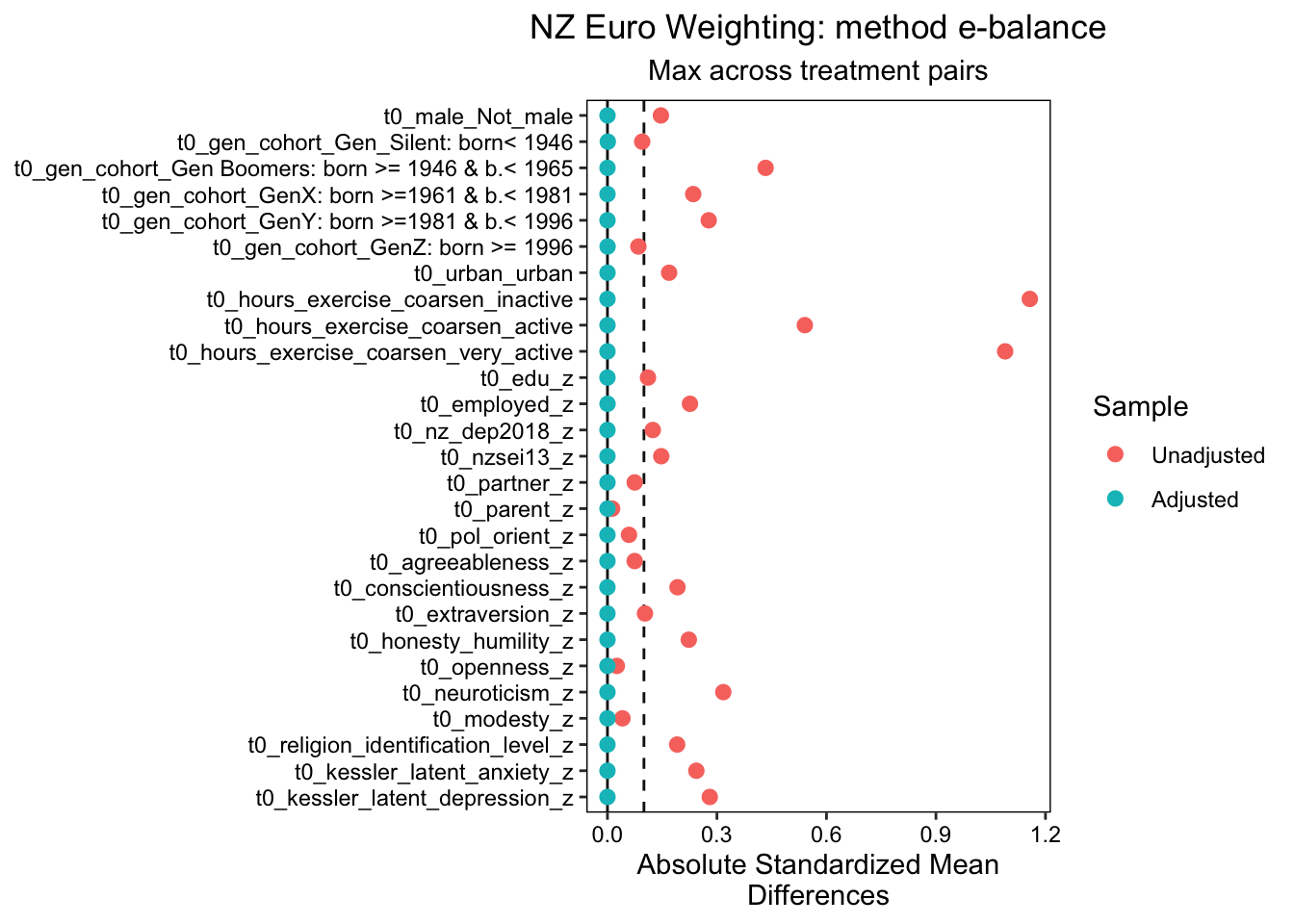
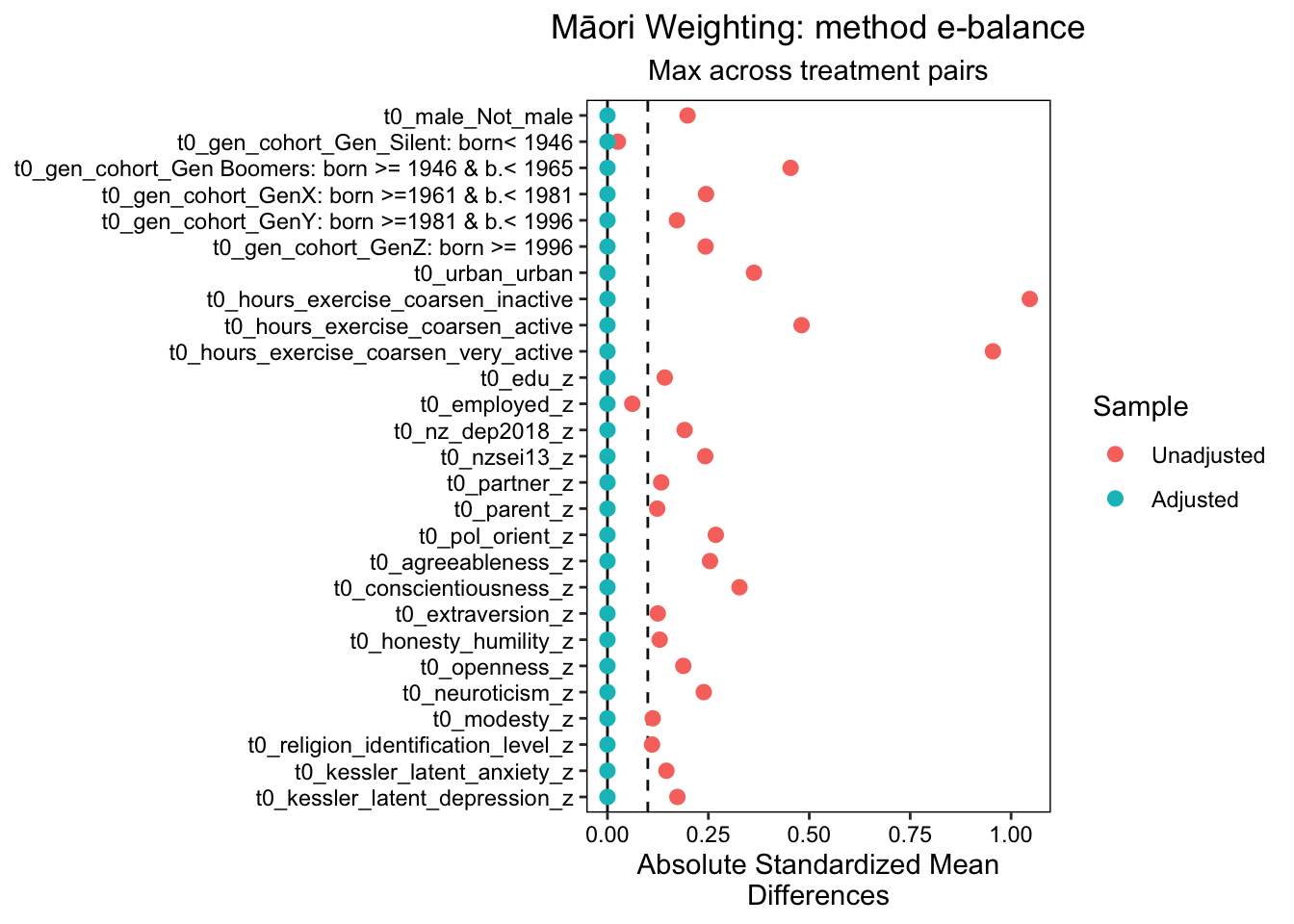
#dt_match_energy <- readRDS(here::here("data", "dt_match_energy"))
dt_match_ebal <- readRDS(here::here("data", "dt_match_ebal"))
#dt_match_ps <- readRDS(here::here("data", "dt_match_ps"))

# next we inspect balance. "Max.Diff.Adj" should ideally be less than .05, but less than .1 is ok. This is the standardised mean difference. The variance ratio should be less than 2. 
# note that if the variables are unlikely to influence the outcome we can be less strict. 

#See: Hainmueller, J. 2012. “Entropy Balancing for Causal Effects: A Multivariate Reweighting Method to Produce Balanced Samples in Observational Studies.” Political Analysis 20 (1): 25–46. https://doi.org/10.1093/pan/mpr025.

# Cole SR, Hernan MA. Constructing inverse probability weights for marginal structural models. American Journal of
# Epidemiology 2008; 168(6):656–664.

# Moving towards best practice when using inverse probability of treatment weighting (IPTW) using the propensity score to estimate causal treatment effects in observational studies
# Peter C. Austin, Elizabeth A. Stuart
# https://onlinelibrary.wiley.com/doi/10.1002/sim.6607

#bal.tab(dt_match_energy$euro)   #  good
bal.tab(dt_match_ebal$euro)   #  best

Balance summary across all treatment pairs
                                                      Type Max.Diff.Adj
t0_male_Not_male                                    Binary       0.0001
t0_gen_cohort_Gen_Silent: born< 1946                Binary       0.0001
t0_gen_cohort_Gen Boomers: born >= 1946 & b.< 1965  Binary       0.0001
t0_gen_cohort_GenX: born >=1961 & b.< 1981          Binary       0.0001
t0_gen_cohort_GenY: born >=1981 & b.< 1996          Binary       0.0001
t0_gen_cohort_GenZ: born >= 1996                    Binary       0.0000
t0_urban_urban                                      Binary       0.0001
t0_hours_exercise_coarsen_inactive                  Binary       0.0000
t0_hours_exercise_coarsen_active                    Binary       0.0000
t0_hours_exercise_coarsen_very_active               Binary       0.0000
t0_edu_z                                           Contin.       0.0000
t0_employed_z                                      Contin.       0.0003
t0_nz_dep2018_z                                    Contin.       0.0000
t0_nzsei13_z                                       Contin.       0.0000
t0_partner_z                                       Contin.       0.0001
t0_parent_z                                        Contin.       0.0001
t0_pol_orient_z                                    Contin.       0.0000
t0_agreeableness_z                                 Contin.       0.0000
t0_conscientiousness_z                             Contin.       0.0000
t0_extraversion_z                                  Contin.       0.0000
t0_honesty_humility_z                              Contin.       0.0001
t0_openness_z                                      Contin.       0.0000
t0_neuroticism_z                                   Contin.       0.0001
t0_modesty_z                                       Contin.       0.0001
t0_religion_identification_level_z                 Contin.       0.0001
t0_kessler_latent_anxiety_z                        Contin.       0.0001
t0_kessler_latent_depression_z                     Contin.       0.0000

Effective sample sizes
           inactive  active very_active
Unadjusted  2880.   3927.       1834.  
Adjusted    1855.89 3659.59     1052.01

#bal.tab(dt_match_ps$euro)   #  not as good

# here we show only the best tab, but you should put all information into an appendix

Results for Maori

# who only Ebal
#bal.tab(dt_match_energy$māori)   #  good
bal.tab(dt_match_ebal$māori)   #  best

Balance summary across all treatment pairs
                                                      Type Max.Diff.Adj
t0_male_Not_male                                    Binary       0.0000
t0_gen_cohort_Gen_Silent: born< 1946                Binary       0.0000
t0_gen_cohort_Gen Boomers: born >= 1946 & b.< 1965  Binary       0.0000
t0_gen_cohort_GenX: born >=1961 & b.< 1981          Binary       0.0000
t0_gen_cohort_GenY: born >=1981 & b.< 1996          Binary       0.0000
t0_gen_cohort_GenZ: born >= 1996                    Binary       0.0000
t0_urban_urban                                      Binary       0.0000
t0_hours_exercise_coarsen_inactive                  Binary       0.0000
t0_hours_exercise_coarsen_active                    Binary       0.0000
t0_hours_exercise_coarsen_very_active               Binary       0.0000
t0_edu_z                                           Contin.       0.0000
t0_employed_z                                      Contin.       0.0001
t0_nz_dep2018_z                                    Contin.       0.0000
t0_nzsei13_z                                       Contin.       0.0000
t0_partner_z                                       Contin.       0.0002
t0_parent_z                                        Contin.       0.0001
t0_pol_orient_z                                    Contin.       0.0000
t0_agreeableness_z                                 Contin.       0.0001
t0_conscientiousness_z                             Contin.       0.0000
t0_extraversion_z                                  Contin.       0.0000
t0_honesty_humility_z                              Contin.       0.0000
t0_openness_z                                      Contin.       0.0000
t0_neuroticism_z                                   Contin.       0.0000
t0_modesty_z                                       Contin.       0.0000
t0_religion_identification_level_z                 Contin.       0.0001
t0_kessler_latent_anxiety_z                        Contin.       0.0000
t0_kessler_latent_depression_z                     Contin.       0.0001

Effective sample sizes
           inactive active very_active
Unadjusted   307.   354.        160.  
Adjusted     220.54 321.09       76.39

#bal.tab(dt_match_ps$māori)   #  not good

# code for summar
sum_e <- summary(dt_match_ebal$euro)
sum_m <- summary(dt_match_ebal$māori)

# summary euro
sum_e

                 Summary of weights

- Weight ranges:

               Min                                  Max
inactive    0.2310 |---------------------------| 7.0511
active      0.5769  |----|                       1.9603
very_active 0.1601 |----------------------|      5.9191

- Units with the 5 most extreme weights by group:
                                               
               6560      9   7209   4878   5105
    inactive 5.1084 5.1312 5.1642 5.3517 7.0511
               3279   1867   4754   2783   7057
      active 1.7467 1.7654 1.7701 1.8692 1.9603
               5977   4293    700   2352   4765
 very_active 5.1495 5.3064 5.4829 5.7273 5.9191

- Weight statistics:

            Coef of Var   MAD Entropy # Zeros
inactive          0.743 0.536   0.212       0
active            0.270 0.248   0.036       0
very_active       0.862 0.637   0.302       0

- Effective Sample Sizes:

           inactive  active very_active
Unweighted  2880.   3927.       1834.  
Weighted    1855.89 3659.59     1052.01

# summary maori
sum_m

                 Summary of weights

- Weight ranges:

               Min                                  Max
inactive    0.2213  |---------------|            3.8101
active      0.3995   |-----|                     1.9800
very_active 0.0719 |---------------------------| 6.2941

- Units with the 5 most extreme weights by group:
                                               
                296    322    355    758    812
    inactive 3.0104  3.407 3.6372 3.7101 3.8101
                 95    783    473    703    699
      active 1.8319 1.8387 1.9395 1.9436   1.98
                745    149     78    226    718
 very_active 4.0921 4.3405 4.4111 4.6833 6.2941

- Weight statistics:

            Coef of Var   MAD Entropy # Zeros
inactive          0.627 0.475   0.170       0
active            0.321 0.264   0.050       0
very_active       1.050 0.732   0.411       0

- Effective Sample Sizes:

           inactive active very_active
Unweighted   307.   354.        160.  
Weighted     220.54 321.09       76.39

love_plot_e <- love.plot(dt_match_ebal$euro,
          binary = "std",
          thresholds = c(m = .1))+ labs(title = "NZ Euro Weighting: method e-balance")

# plot
love_plot_e

love_plot_m <- love.plot(dt_match_ebal$māori,
          binary = "std",
          thresholds = c(m = .1)) + labs(title = "Māori Weighting: method e-balance")
# plot
love_plot_m

Example Summary NZ Euro Propensity scores.

We estimated propensity score analysis using entropy balancing, energy balancing and traditional propensity scores. Of these approaches, entropy balancing provided the best balance. The results indicate an excellent balance across all variables, with Max.Diff.Adj values significantly below the target threshold of 0.05 across a range of binary and continuous baseline confounders, including gender, generation cohort, urban_location, exercise hours (coarsened, baseline), education, employment status, depression, anxiety, and various personality traits. The Max.Diff.Adj values for all variables were well below the target threshold of 0.05, with most variables achieving a Max.Diff.Adj of 0.0001 or lower. This indicates a high level of balance across all treatment pairs.

The effective sample sizes were also adjusted using entropy balancing. The unadjusted sample sizes for the inactive, active, and very active groups were 2880, 3927, and 1834, respectively. After adjustment, the effective sample sizes were reduced to 1855.89, 3659.59, and 1052.01, respectively.

The weight ranges for the inactive, active, and very active groups varied, with the inactive group showing the widest range (0.2310 to 7.0511) and the active group showing the narrowest range (0.5769 to 1.9603). Despite these variations, the coefficient of variation, mean absolute deviation (MAD), and entropy were all within acceptable limits for each group, indicating a good balance of weights.

We also identified the units with the five most extreme weights by group. These units exhibited higher weights compared to the rest of the units in their respective groups, but they did not significantly affect the overall balance of weights.

We plotted these results using love plots, visually confirming both the balance in the propensity score model using entropy balanced weights, and the imbalance in the model that does not adjust for baseline confounders.

Overall, these findings support the use of entropy balancing in propensity score analysis to ensure a balanced distribution of covariates across treatment groups, conditional on the measured covariates included in the model.

Example Summary Maori Propensity scores.

Results:

The entropy balancing method was also the best performing method that was applied to a subgroup analysis of the Māori population. Similar to the NZ European subgroup analysis, the method achieved a high level of balance across all treatment pairs for the Māori subgroup. The Max.Diff.Adj values for all variables were well below the target threshold of 0.05, with most variables achieving a Max.Diff.Adj of 0.0001 or lower. This indicates a high level of balance across all treatment pairs for the Māori subgroup.

The effective sample sizes for the Māori subgroup were also adjusted using entropy balancing. The unadjusted sample sizes for the inactive, active, and very active groups were 307, 354, and 160, respectively. After adjustment, the effective sample sizes were reduced to 220.54, 321.09, and 76.39, respectively

The weight ranges for the inactive, active, and very active groups in the Māori subgroup varied, with the inactive group showing the widest range (0.2213 to 3.8101) and the active group showing the narrowest range (0.3995 to 1.9800). Despite these variations, the coefficient of variation, mean absolute deviation (MAD), and entropy were all within acceptable limits for each group, indicating a good balance of weights.

The study also identified the units with the five most extreme weights by group for the Māori subgroup. These units exhibited higher weights compared to the rest of the units in their respective groups, but they did not significantly affect the overall balance of weights.

In conclusion, the results of the Māori subgroup analysis are consistent with the overall analysis. The entropy balancing method achieved a high level of balance across all treatment pairs, with Max.Diff.Adj values significantly below the target threshold. These findings support the use of entropy balancing in propensity score analysis to ensure a balanced distribution of covariates across treatment groups, even in subgroup analyses.

More data wrangling

Note that we need to attach the weights from the propensity score model back to the data.

However, because our weighting analysis estimates a model for the exposure, we only need to do this analysis once, no matter how many outcomes we investigate. So there’s a little good news.

# prepare nz_euro data
dt_ref_e <- subset(dt, t0_eth_cat == "euro") # original data subset only nz europeans

# add weights
dt_ref_e$weights <- dt_match_ebal$euro$weights # get weights from the ps matching model,add to data

# prepare maori data
dt_ref_m <- subset(dt, t0_eth_cat == "māori")# original data subset only maori

# add weights
dt_ref_m$weights <- dt_match_ebal$māori$weights # get weights from the ps matching model, add to data

# combine data into one data frame
dt_ref_all <- rbind(dt_ref_e, dt_ref_m) # combine the data into one dataframe.

Table of Subgroup Results plus Evalues

I’ve created functions for reporting results so you can use this code, changing it to suit your analysis.

# return stored estimates 
sim_estimand_all_e <- readRDS(here::here("data","sim_estimand_all_e"))
sim_estimand_all_m<- readRDS(here::here("data","sim_estimand_all_m"))

# create individual summaries 
sum_e <- summary(sim_estimand_all_e)
sum_m <- summary(sim_estimand_all_m)


# create individual tables
tab_e <- sub_tab_ate(sum_e, new_name = "NZ Euro Anxiety")

Warning: There was 1 warning in `dplyr::mutate()`.
ℹ In argument: `across(where(is.numeric), round, digits = 4)`.
Caused by warning:
! The `...` argument of `across()` is deprecated as of dplyr 1.1.0.
Supply arguments directly to `.fns` through an anonymous function instead.

  # Previously
  across(a:b, mean, na.rm = TRUE)

  # Now
  across(a:b, \(x) mean(x, na.rm = TRUE))

tab_m <- sub_tab_ate(sum_m, new_name = "Māori Anxiety")

Confidence interval crosses the true value, so its E-value is 1.

# expand tables 
plot_e <- sub_group_tab(tab_e, type= "RD")
plot_m <- sub_group_tab(tab_m, type= "RD")

big_tab <- rbind(plot_e,plot_m)


# table for anxiety outcome --format as "markdown" if you are using quarto documents
big_tab |> 
  kbl(format="markdown")

group	E[Y(1)]-E[Y(0)]	2.5 %	97.5 %	E_Value	E_Val_bound	Estimate	estimate_lab
NZ Euro Anxiety	-0.077	-0.131	-0.022	1.352	1.167	negative	-0.077 (-0.131–0.022) [EV 1.352/1.167]
Māori Anxiety	0.027	-0.114	0.188	1.183	1.000	unreliable	0.027 (-0.114-0.188) [EV 1.183/1]

Graph of the result

I’ve create a function you can use to graph your results. Here is the code, adjust to suit.

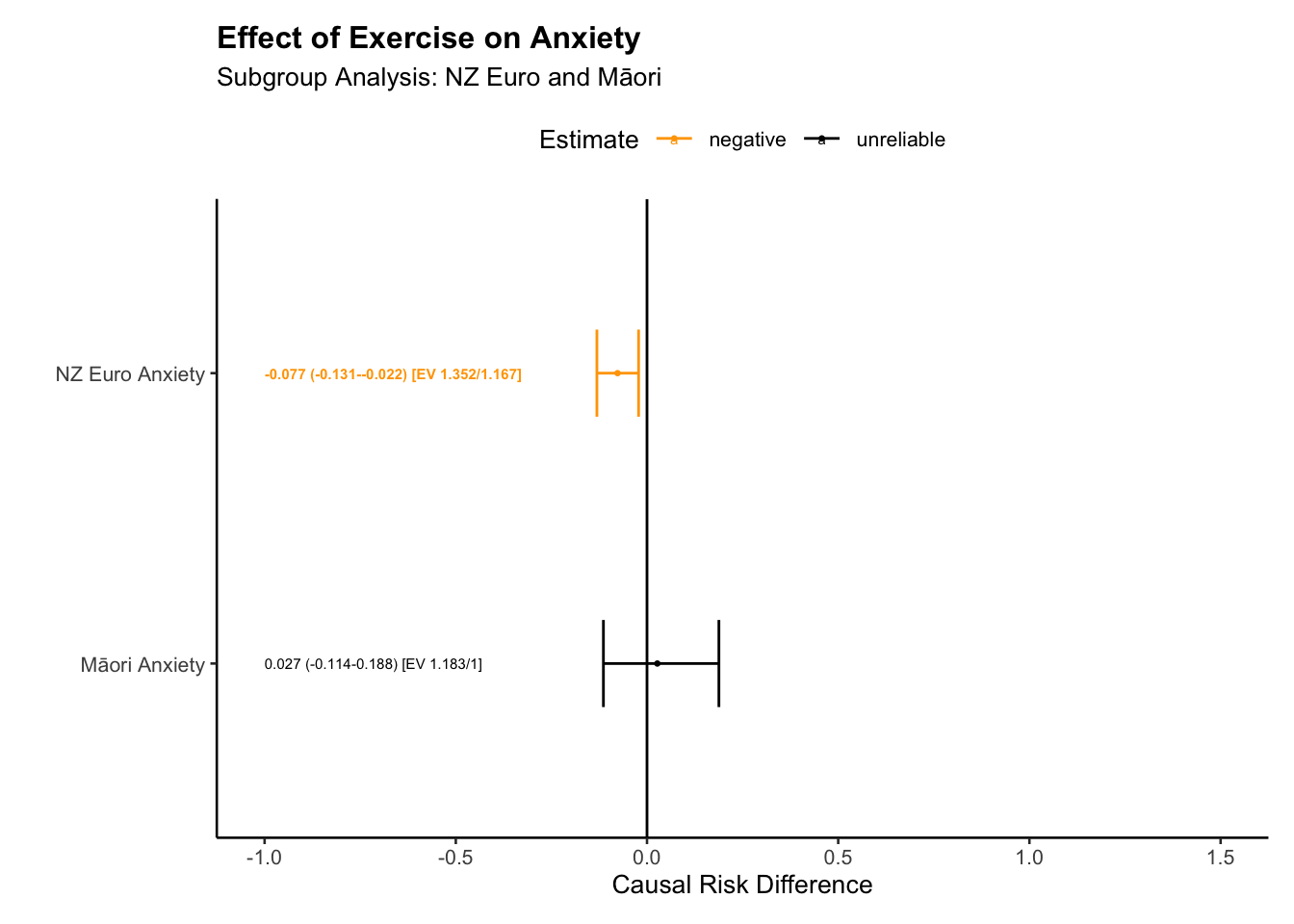
# group tables
sub_group_plot_ate(big_tab, title = "Effect of Exercise on Anxiety", subtitle = "Subgroup Analysis: NZ Euro and Māori", xlab = "Groups", ylab = "Effects",
                 x_offset = -1,
                           x_lim_lo = -1,
                           x_lim_hi = 1.5)

Report the anxiety result.

For the New Zealand European group, our results suggest that exercise potentially reduces anxiety, with an estimated causal contrast value (E[Y(1)]-E[Y(0)]) of -0.077. The associated confidence interval, ranging from -0.131 to -0.022, does not cross zero, providing more certainty in our estimate.

E-values quantify the minimum strength of association that an unmeasured confounding variable would need to have with both the treatment and outcome, to fully explain away our observed effect. In this case, any unmeasured confounder would need to be associated with both exercise and anxiety reduction, with a risk ratio of at least 1.352 to explain away the observed effect, and at least 1.167 to shift the confidence interval to include a null effect.

Turning to the Māori group, the data suggest a possible reducing effect of exercise on anxiety, with a causal contrast value of 0.027. Yet, the confidence interval for this estimate (-0.114 to 0.188) also crosses zero, indicating similar uncertainties. An unmeasured confounder would need to have a risk ratio of at least 1.183 with both exercise and anxiety to account for our observed effect, and a risk ratio of at least 1 to render the confidence interval inclusive of a null effect.

Thus, while our analysis suggests that exercise could potentially reduce anxiety in both New Zealand Europeans and Māori, we advise caution in interpretation. The confidence intervals crossing zero reflect substantial uncertainties, and the possible impact of unmeasured confounding factors further complicates the picture.

Here’s a function that will do much of this work for you. However, you’ll need to adjust it, and supply your own interpretation.

#|label: interpretation function
#| eval: false
interpret_results_subgroup <- function(df, outcome, exposure) {
  df <- df %>%
    mutate(
      report = case_when(
        E_Val_bound > 1.2 & E_Val_bound < 2 ~ paste0(
          "For the ", group, ", our results suggest that ", exposure, " may potentially influence ", outcome, ", with an estimated causal contrast value (E[Y(1)]-E[Y(0)]) of ", `E[Y(1)]-E[Y(0)]`, ".\n",
          "The associated confidence interval, ranging from ", `2.5 %`, " to ", `97.5 %`, ", does not cross zero, providing more certainty in our estimate. ",
          "The E-values indicate that any unmeasured confounder would need to have a minimum risk ratio of ", E_Value, " with both the treatment and outcome to explain away the observed effect, and a minimum risk ratio of ", E_Val_bound, " to shift the confidence interval to include the null effect. This suggests stronger confidence in our findings."
        ),
        E_Val_bound >= 2 ~ paste0(
          "For the ", group, ", our results suggest that ", exposure, " may potentially influence ", outcome, ", with an estimated causal contrast value (E[Y(1)]-E[Y(0)]) of ", `E[Y(1)]-E[Y(0)]`, ".\n",
          "The associated confidence interval, ranging from ", `2.5 %`, " to ", `97.5 %`, ", does not cross zero, providing more certainty in our estimate. ",
          "With an observed risk ratio of RR = ", E_Value, ", an unmeasured confounder that was associated with both the outcome and the exposure by a risk ratio of ", E_Val_bound, "-fold each, above and beyond the measured confounders, could explain away the estimate, but weaker joint confounder associations could not; to move the confidence interval to include the null, an unmeasured confounder that was associated with the outcome and the exposure by a risk ratio of ", E_Val_bound, "-fold each could do so, but weaker joint confounder associations could not. Here we find stronger evidence that the result is robust to unmeasured confounding."
        ),
        E_Val_bound < 1.2 & E_Val_bound > 1 ~ paste0(
          "For the ", group, ", our results suggest that ", exposure, " may potentially influence ", outcome, ", with an estimated causal contrast value (E[Y(1)]-E[Y(0)]) of ", `E[Y(1)]-E[Y(0)]`, ".\n",
          "The associated confidence interval, ranging from ", `2.5 %`, " to ", `97.5 %`, ", does not cross zero, providing more certainty in our estimate. ",
          "The E-values indicate that any unmeasured confounder would need to have a minimum risk ratio of ", E_Value, " with both the treatment and outcome to explain away the observed effect, and a minimum risk ratio of ", E_Val_bound, " to shift the confidence interval to include the null effect. This suggests we should interpret these findings with caution given uncertainty in the model."
        ),
        E_Val_bound == 1 ~ paste0(
          "For the ", group, ", the data suggests a potential effect of ", exposure, " on ", outcome, ", with a causal contrast value of ", `E[Y(1)]-E[Y(0)]`, ".\n",
          "However, the confidence interval for this estimate, ranging from ", `2.5 %`," to ", `97.5 %`, ", crosses zero, indicating considerable uncertainties. The E-values indicate that an unmeasured confounder that is associated with both the ", outcome, " and the ", exposure, " by a risk ratio of ", E_Value, " could explain away the observed associations, even after accounting for the measured confounders. ",
          "This finding further reduces confidence in a true causal effect. Hence, while the estimates suggest a potential effect of ", exposure, " on ", outcome, " for the ", group, ", the substantial uncertainty and possible influence of unmeasured confounders mean these findings should be interpreted with caution."
        )
      )
    )
  return(df$report)
}

You run the function like this:

interpret_results_subgroup(big_tab, outcome = "Anxiety", exposure = "Excercise")

[1] "For the NZ Euro Anxiety, our results suggest that Excercise may potentially influence Anxiety, with an estimated causal contrast value (E[Y(1)]-E[Y(0)]) of -0.077.\nThe associated confidence interval, ranging from -0.131 to -0.022, does not cross zero, providing more certainty in our estimate. The E-values indicate that any unmeasured confounder would need to have a minimum risk ratio of 1.352 with both the treatment and outcome to explain away the observed effect, and a minimum risk ratio of 1.167 to shift the confidence interval to include the null effect. This suggests we should interpret these findings with caution given uncertainty in the model."                                                                                                                                      
[2] "For the Māori Anxiety, the data suggests a potential effect of Excercise on Anxiety, with a causal contrast value of 0.027.\nHowever, the confidence interval for this estimate, ranging from -0.114 to 0.188, crosses zero, indicating considerable uncertainties. The E-values indicate that an unmeasured confounder that is associated with both the Anxiety and the Excercise by a risk ratio of 1.183 could explain away the observed associations, even after accounting for the measured confounders. This finding further reduces confidence in a true causal effect. Hence, while the estimates suggest a potential effect of Excercise on Anxiety for the Māori Anxiety, the substantial uncertainty and possible influence of unmeasured confounders mean these findings should be interpreted with caution."

Easy!

Estimate the subgroup contrast

# calculated above
est_all_anxiety <- readRDS( here::here("data","est_all_anxiety"))

# make the sumamry into a dataframe so we can make a table
df <- as.data.frame(summary(est_all_anxiety))

# get rownames for selecting the correct row
df$RowName <- row.names(df)

# select the correct row -- the group contrast
filtered_df <- df |> 
  dplyr::filter(RowName == "RD_m - RD_e") 


# pring the filtered data frame
library(kableExtra)
filtered_df  |> 
  select(-RowName) |> 
  kbl(digits = 3) |> 
  kable_material(c("striped", "hover"))

	Estimate	2.5 %	97.5 %
RD_m - RD_e	0.104	-0.042	0.279

Another option for making the table using markdown. This would be useful if you were writing your article using qaurto.

filtered_df  |> 
  select(-RowName) |> 
  kbl(digits = 3, format = "markdown")

	Estimate	2.5 %	97.5 %
RD_m - RD_e	0.104	-0.042	0.279

Report result along the following lines:

The estimated reduction of anxiety from exercise is higher overall for New Zealand Europeans (RD_e) compared to Māori (RD_m). This is indicated by the estimated risk difference (RD_m - RD_e) of 0.104. However, there is uncertainty in this estimate, as the confidence interval (-0.042 to 0.279) crosses zero. This indicates that we cannot be confident that the difference in anxiety reduction between New Zealand Europeans and Māori is reliable. It’s possible that the true difference could be zero or even negative, suggesting higher anxiety reduction for Māori. Thus, while there’s an indication of higher anxiety reduction for New Zealand Europeans, the uncertainty in the estimate means we should interpret this difference with caution.

Depression Analysis and Results

### SUBGROUP analysis
dt_ref_all <- readRDS(here::here("data", "dt_ref_all"))
# get column names
baseline_vars_reflective_propensity <- dt|>
  dplyr::select(starts_with("t0"), -t0_eth_cat) |> colnames()
df <-  dt_ref_all
Y <-  "t2_kessler_latent_depression_z"
X <- "t1_hours_exercise_coarsen" # already defined above
baseline_vars = baseline_vars_reflective_propensity
treat_0 = "inactive"
treat_1 = "very_active"
estimand = "ATE"
scale = "RD"
nsims = 1000
family = "gaussian"
continuous_X = FALSE
splines = FALSE
cores = parallel::detectCores()
S = "t0_eth_cat"

# not we interact the subclass X treatment X covariates

formula_str <-
  paste(
    Y,
    "~",
    S,
    "*",
    "(",
    X ,
    "*",
    "(",
    paste(baseline_vars_reflective_propensity, collapse = "+"),
    ")",
    ")"
  )

# fit model
fit_all_dep  <- glm(
  as.formula(formula_str),
  weights = weights,
  # weights = if (!is.null(weight_var)) weight_var else NULL,
  family = family,
  data = df
)


# coefs <- coef(fit_all_dep)
# table(is.na(coefs))#   
# insight::get_varcov(fit_all_all)

# simulate coefficients
conflicts_prefer(clarify::sim)
sim_model_all <- sim(fit_all_dep, n = nsims, vcov = "HC1")


# simulate effect as modified in europeans
sim_estimand_all_e_d <- sim_ame(
  sim_model_all,
  var = X,
  cl = cores,
  subset = t0_eth_cat == "euro",
  verbose = TRUE)


# note contrast of interest
sim_estimand_all_e_d <-
  transform(sim_estimand_all_e_d, RD = `E[Y(very_active)]` - `E[Y(inactive)]`)


# simulate effect as modified in māori
sim_estimand_all_m_d <- sim_ame(
  sim_model_all,
  var = X,
  cl = cores,
  subset = t0_eth_cat == "māori",
  verbose = TRUE
)

# combine
sim_estimand_all_m_d <-
  transform(sim_estimand_all_m_d, RD = `E[Y(very_active)]` - `E[Y(inactive)]`)


# summary
#summary(sim_estimand_all_e_d)
#summary(sim_estimand_all_m_d)

# rearrange
names(sim_estimand_all_e_d) <-
  paste(names(sim_estimand_all_e_d), "e", sep = "_")

names(sim_estimand_all_m_d) <-
  paste(names(sim_estimand_all_m_d), "m", sep = "_")


est_all_d <- cbind(sim_estimand_all_m_d, sim_estimand_all_e_d)
est_all_d <- transform(est_all_d, `RD_m - RD_e` = RD_m - RD_e)
saveRDS(sim_estimand_all_m_d, here::here("data", "sim_estimand_all_m_d"))
saveRDS(sim_estimand_all_e_d, here::here("data", "sim_estimand_all_e_d"))

Report anxiety results

# return stored estimates 
sim_estimand_all_e_d <- readRDS(here::here("data","sim_estimand_all_e_d"))
sim_estimand_all_m_d<- readRDS(here::here("data","sim_estimand_all_m_d"))

# create individual summaries 
sum_e_d <- summary(sim_estimand_all_e_d)
sum_m_d <- summary(sim_estimand_all_m_d)


# create individual tables
tab_ed <- sub_tab_ate(sum_e_d, new_name = "NZ Euro Depression")

Confidence interval crosses the true value, so its E-value is 1.

tab_md <- sub_tab_ate(sum_m_d, new_name = "Māori Depression")

Confidence interval crosses the true value, so its E-value is 1.

# expand tables 
plot_ed <- sub_group_tab(tab_ed, type= "RD")
plot_md <- sub_group_tab(tab_md, type= "RD")

big_tab_d <- rbind(plot_ed,plot_md)


# table for anxiety outcome --format as "markdown" if you are using quarto documents
big_tab_d |> 
  kbl(format="markdown")

group	E[Y(1)]-E[Y(0)]	2.5 %	97.5 %	E_Value	E_Val_bound	Estimate	estimate_lab
NZ Euro Depression	-0.039	-0.099	0.019	1.231	1	unreliable	-0.039 (-0.099-0.019) [EV 1.231/1]
Māori Depression	0.028	-0.125	0.176	1.190	1	unreliable	0.028 (-0.125-0.176) [EV 1.19/1]

Graph Anxiety result

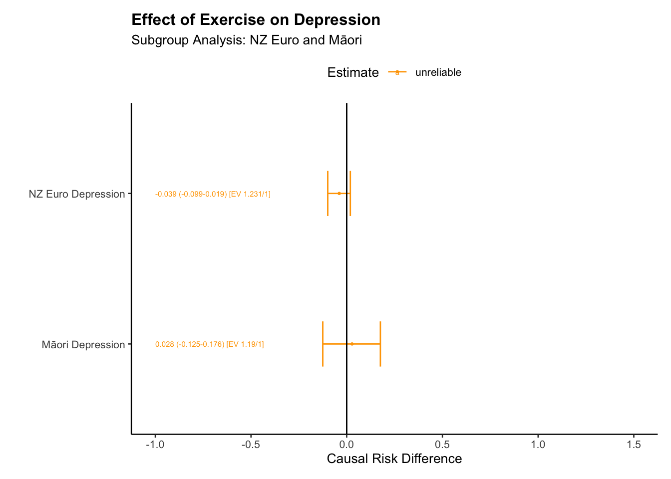
# group tables
sub_group_plot_ate(big_tab_d, title = "Effect of Exercise on Depression", subtitle = "Subgroup Analysis: NZ Euro and Māori", xlab = "Groups", ylab = "Effects",
                 x_offset = -1,
                           x_lim_lo = -1,
                           x_lim_hi = 1.5)

Interpretation

Use the function, again, modify the outputs to fit with your study and results and provide your own interpretation.

interpret_results_subgroup(big_tab_d, exposure = "Exercise", outcome = "Depression")

[1] "For the NZ Euro Depression, the data suggests a potential effect of Exercise on Depression, with a causal contrast value of -0.039.\nHowever, the confidence interval for this estimate, ranging from -0.099 to 0.019, crosses zero, indicating considerable uncertainties. The E-values indicate that an unmeasured confounder that is associated with both the Depression and the Exercise by a risk ratio of 1.231 could explain away the observed associations, even after accounting for the measured confounders. This finding further reduces confidence in a true causal effect. Hence, while the estimates suggest a potential effect of Exercise on Depression for the NZ Euro Depression, the substantial uncertainty and possible influence of unmeasured confounders mean these findings should be interpreted with caution."
[2] "For the Māori Depression, the data suggests a potential effect of Exercise on Depression, with a causal contrast value of 0.028.\nHowever, the confidence interval for this estimate, ranging from -0.125 to 0.176, crosses zero, indicating considerable uncertainties. The E-values indicate that an unmeasured confounder that is associated with both the Depression and the Exercise by a risk ratio of 1.19 could explain away the observed associations, even after accounting for the measured confounders. This finding further reduces confidence in a true causal effect. Hence, while the estimates suggest a potential effect of Exercise on Depression for the Māori Depression, the substantial uncertainty and possible influence of unmeasured confounders mean these findings should be interpreted with caution."

Estimate the subgroup contrast

# calculated above
est_all_d <- readRDS( here::here("data","est_all_d"))

# make the sumamry into a dataframe so we can make a table
dfd <- as.data.frame(summary(est_all_d))

# get rownames for selecting the correct row
dfd$RowName <- row.names(dfd)

# select the correct row -- the group contrast
filtered_dfd <- dfd |> 
  dplyr::filter(RowName == "RD_m - RD_e") 


# Print the filtered data frame
library(kableExtra)
filtered_dfd  |> 
  select(-RowName) |> 
  kbl(digits = 3) |> 
  kable_material(c("striped", "hover"))

	Estimate	2.5 %	97.5 %
RD_m - RD_e	0.068	-0.09	0.229

Reporting might be:

The estimated reduction of depression from exercise is higher overall for New Zealand Europeans (RD_e) compared to Māori (RD_m). This is suggested by the estimated risk difference (RD_m - RD_e) of 0.068. However, there is a degree of uncertainty in this estimate, as the confidence interval (-0.09 to 0.229) crosses zero. This suggests that we cannot be confident that the difference in depression reduction between New Zealand Europeans and Māori is statistically significant. It’s possible that the true difference could be zero or even negative, implying a greater depression reduction for Māori than New Zealand Europeans. Thus, while the results hint at a larger depression reduction for New Zealand Europeans, the uncertainty in this estimate urges us to interpret this difference with caution.

Discusion

You’ll need to do this yourself. Here’s a start:

In our study, we employed a robust statistical method that helps us estimate the impact of exercise on reducing anxiety among different population groups – New Zealand Europeans and Māori. This method has the advantage of providing reliable results even if our underlying assumptions aren’t entirely accurate – a likely scenario given the complexity of real-world data. However, this robustness comes with a trade-off: it gives us wider ranges of uncertainty in our estimates. This doesn’t mean the analysis is flawed; rather, it accurately represents our level of certainty given the data we have.

Exercise and Anxiety

Our analysis suggests that exercise may have a greater effect in reducing anxiety among New Zealand Europeans compared to Māori. This conclusion comes from our primary causal estimate, the risk difference, which is 0.104. However, it’s crucial to consider our uncertainty in this value. We represent this uncertainty as a range, also known as a confidence interval. In this case, the interval ranges from -0.042 to 0.279. What this means is, given our current data and method, the true effect could plausibly be anywhere within this range. While our best estimate shows a higher reduction in anxiety for New Zealand Europeans, the range of plausible values includes zero and even negative values. This implies that the true effect could be no difference between the two groups or even a higher reduction in Māori. Hence, while there’s an indication of a difference, we should interpret it cautiously given the wide range of uncertainty.

Thus, although our analysis points towards a potential difference in how exercise reduces anxiety among these groups, the level of uncertainty means we should be careful about drawing firm conclusions. More research is needed to further explore these patterns.

Exercise and Depression

In addition to anxiety, we also examined the effect of exercise on depression. We do not find evidence for reduction of depression from exercise in either group. We do not find evidence for the effect of weekly exercise – as self-reported – on depression.

Proviso

It is important to bear in mind that statistical results are only one piece of a larger scientific puzzle about the relationship between excercise and well-being. Other pieces include understanding the context, incorporating subject matter knowledge, and considering the implications of the findings. In the present study, wide confidence intervals suggest the possibility of considerable individual differences.\dots nevertheless, \dots

Exercises

Generate a Kessler 6 binary score (Not Depressed vs. Moderately or Severely Depressed)

and also:

Create a variable for the log of exercise hour
Take Home: estimate whether exercise causally affects nervousness, using the single item of the kessler 6 score. Briefly write up your results.

Appendix: MG-CFA

CFA for Kessler 6

We have learned how to do confirmatory factor analysis. Let’s put this knowledge to use but clarifying the underlying factor structure of Kessler-6

The code below will:

Load required packages.
Select the Kessler 6 items
Check whether there is sufficient correlation among the variables to support factor analysis.

# select the columns we need. 
dt_only_k6 <- dt_start |> select(kessler_depressed, kessler_effort,kessler_hopeless,
                                 kessler_worthless, kessler_nervous,
                                 kessler_restless)


# check factor structure
performance::check_factorstructure(dt_only_k6)

# Is the data suitable for Factor Analysis?


  - Sphericity: Bartlett's test of sphericity suggests that there is sufficient significant correlation in the data for factor analysis (Chisq(15) = 70564.23, p < .001).
  - KMO: The Kaiser, Meyer, Olkin (KMO) overall measure of sampling adequacy suggests that data seems appropriate for factor analysis (KMO = 0.86). The individual KMO scores are: kessler_depressed (0.83), kessler_effort (0.89), kessler_hopeless (0.85), kessler_worthless (0.85), kessler_nervous (0.88), kessler_restless (0.85).

The code below will allow us to explore the factor structure, on the assumption of n = 3 factors.

# exploratory factor analysis
# explore a factor structure made of 3 latent variables
efa <- psych::fa(dt_only_k6, nfactors = 3) %>%
  model_parameters(sort = TRUE, threshold = "max")

Loading required namespace: GPArotation

efa

# Rotated loadings from Factor Analysis (oblimin-rotation)

Variable          | MR1  | MR2  | MR3  | Complexity | Uniqueness
----------------------------------------------------------------
kessler_depressed | 0.85 |      |      |    1.01    |    0.33   
kessler_worthless | 0.79 |      |      |    1.00    |    0.35   
kessler_hopeless  | 0.75 |      |      |    1.02    |    0.33   
kessler_nervous   |      | 1.00 |      |    1.00    |  5.00e-03 
kessler_restless  |      |      | 0.69 |    1.02    |    0.52   
kessler_effort    |      |      | 0.48 |    1.66    |    0.50   

The 3 latent factors (oblimin rotation) accounted for 66.05% of the total variance of the original data (MR1 = 35.14%, MR2 = 17.17%, MR3 = 13.73%).

This output describes an exploratory factor analysis (EFA) with 3 factors conducted on the Kessler 6 (K6) scale data. The K6 scale is used to measure psychological distress.

The analysis identifies three latent factors, labeled MR1, MR2, and MR3, which collectively account for 66.05% of the variance in the K6 data. The factors MR1, MR2, and MR3 explain 35.14%, 17.17%, and 13.73% of the variance respectively.

Factor loadings, indicating the strength and direction of the relationship between the K6 items and the latent factors, are as follows:

Factor MR1 is strongly associated with ‘kessler_depressed’, ‘kessler_worthless’, and ‘kessler_hopeless’ with loadings of 0.85, 0.79, and 0.75 respectively.
Factor MR2 is exclusively linked with ‘kessler_nervous’ with a loading of 1.00.
Factor MR3 relates to ‘kessler_restless’ and ‘kessler_effort’ with loadings of 0.69 and 0.48 respectively.

The ‘Uniqueness’ values show the proportion of each variable’s variance that isn’t shared with the other variables.

The ‘Complexity’ values give a measure of how each item loads on more than one factor. All the items are either loading exclusively on one factor (complexity=1.00) or slightly more than one factor. ‘kessler_effort’ with complexity of 1.66 shows it’s the item most shared between the factors.

The analysis suggests these K6 items measure may measure three somewhat distinct, yet related, factors of psychological distress.

However, the meaning of these factors would need to be interpreted in the context of the variables and the theoretical framework of the study.

Notably, there are many many theoretical frameworks for in measurement theory. Here is a brief description of the different conclusions one might make, depending on one’s preferred theory.

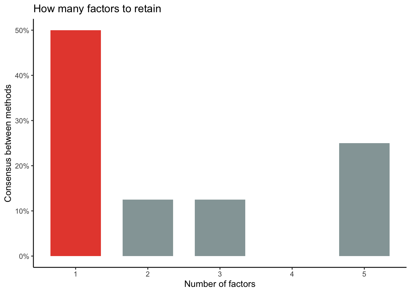
Code

n <- n_factors(dt_only_k6)

# plot
plot(n) + theme_classic()

Confirmatory factor analysis (ignoring groups)

# first partition the data 
part_data <- datawizard::data_partition(dt_only_k6, traing_proportion = .7, seed = 123)


# set up training data
training <- part_data$p_0.7
test <- part_data$test


# one factor model
structure_k6_one <- psych::fa(training, nfactors = 1) |>
  efa_to_cfa()

# two factor model model
structure_k6_two <- psych::fa(training, nfactors = 2) |>
  efa_to_cfa()

# three factor model
structure_k6_three <- psych::fa(training, nfactors = 3) %>%
  efa_to_cfa()

# inspect models
structure_k6_one

# Latent variables
MR1 =~ kessler_depressed + kessler_effort + kessler_hopeless + kessler_worthless + kessler_nervous + kessler_restless + .row_id

structure_k6_two

# Latent variables
MR1 =~ kessler_depressed + kessler_hopeless + kessler_worthless
MR2 =~ kessler_effort + kessler_nervous + kessler_restless + .row_id

structure_k6_three

# Latent variables
MR1 =~ kessler_depressed + kessler_effort + kessler_hopeless + kessler_worthless
MR2 =~ kessler_restless
MR3 =~ kessler_nervous + .row_id

Next we perform the confirmatory factor analysis.

# fit and compare models

# one latent model
one_latent <-
  suppressWarnings(lavaan::cfa(structure_k6_one, data = test))

# two latents model
two_latents <-
  suppressWarnings(lavaan::cfa(structure_k6_two, data = test))

# three latents model
three_latents <-
  suppressWarnings(lavaan::cfa(structure_k6_three, data = test))


# compare models
compare <-
  performance::compare_performance(one_latent, two_latents, three_latents, verbose = FALSE)

# view as html table
as.data.frame(compare) |>
  kbl(format = "markdown")

Name	Model	Chi2	Chi2_df	Baseline	Baseline_df	GFI	AGFI	NFI	NNFI	CFI	RMSEA	RMSEA_CI_low	RMSEA_CI_high	p_RMSEA	RMR	SRMR	RFI	PNFI	IFI	RNI	Loglikelihood	AIC	AIC_wt	BIC	BIC_wt	BIC_adjusted
one_latent	lavaan	1359.7168	14	159746.19	21	0.9533955	0.9067909	0.9914883	0.9873622	0.9915748	0.1033455	0.0987385	0.1080285	0.0000000	36.00334	0.0493327	0.9872324	0.6609922	0.9915752	0.9915748	-151483.7	302995.3	0	303094.8	0	303050.3
two_latents	lavaan	317.9709	13	30915.77	21	0.9900793	0.9786322	0.9897149	0.9840541	0.9901287	0.0510548	0.0462789	0.0559908	0.3499758	36.31236	0.0226983	0.9833857	0.6126807	0.9901313	0.9901287	-150962.8	301955.6	1	302062.2	1	302014.5
three_latents	lavaan	747.8723	12	20903.30	21	0.9763317	0.9447739	0.9642223	0.9383317	0.9647609	0.0825447	0.0775761	0.0876237	0.0000000	37.13824	0.0377955	0.9373890	0.5509842	0.9647761	0.9647609	-151177.7	302387.5	0	302501.2	0	302450.3

This table provides the results of three different Confirmatory Factor Analysis (CFA) models: one that specifies a single latent factor, one that specifies two latent factors, and one that specifies three latent factors. The results include a number of goodness-of-fit statistics, which can be used to assess how well each model fits the data.

One_latent CFA:

This model assumes that there is only one underlying latent factor contributing to all variables. This model has a chi-square statistic of 1359.7 with 14 degrees of freedom, which is highly significant (p<0.001), indicating a poor fit of the model to the data. Other goodness-of-fit indices like GFI, AGFI, NFI, NNFI, and CFI are all high (above 0.9), generally indicating good fit, but these indices can be misleading in the presence of large sample sizes. RMSEA is above 0.1 which indicates a poor fit. The SRMR is less than 0.08 which suggests a good fit, but given the high Chi-square and RMSEA values, we can’t solely rely on this index. The Akaike information criterion (AIC), Bayesian information criterion (BIC) and adjusted BIC are used for comparing models, with lower values indicating better fit.

Two_latents CFA

This model assumes that there are two underlying latent factors. The chi-square statistic is lower than the one-factor model (317.97 with 13 df), suggesting a better fit. The p-value is still less than 0.05, indicating a statistically significant chi-square, which typically suggests a poor fit. However, all other fit indices (GFI, AGFI, NFI, NNFI, and CFI) are above 0.9 and the RMSEA is 0.051, which generally indicate good fit. The SRMR is also less than 0.08 which suggests a good fit. This model has the lowest AIC and BIC values among the three models, indicating the best fit according to these criteria.

Three_latents CFA

This model assumes three underlying latent factors. The chi-square statistic is 747.87 with 12 df, higher than the two-factor model, suggesting a worse fit to the data. Other fit indices such as GFI, AGFI, NFI, NNFI, and CFI are below 0.97 and the RMSEA is 0.083, which generally indicate acceptable but not excellent fit. The SRMR is less than 0.08 which suggests a good fit. The AIC and BIC values are higher than the two-factor model but lower than the one-factor model, indicating a fit that is better than the one-factor model but worse than the two-factor model.

Based on these results, the two-latents model seems to provide the best fit to the data among the three models, according to most of the fit indices and the AIC and BIC. Note, all models have significant chi-square statistics, which suggests some degree of misfit. It’s also important to consider the substantive interpretation of the factors, to make sure the model makes sense theoretically.

Multi-group Confirmatory Factor Analysis

This script runs multi-group confirmatory factor analysis (MG-CFA)

# select needed columns plus 'ethnicity'
# filter dataset for only 'euro' and 'maori' ethnic categories
dt_eth_k6_eth <- dt_start |> 
  filter(eth_cat == "euro" | eth_cat == "maori") |> 
  select(kessler_depressed, kessler_effort,kessler_hopeless,
         kessler_worthless, kessler_nervous,
         kessler_restless, eth_cat)

# partition the dataset into training and test subsets
# stratify by ethnic category to ensure balanced representation
part_data_eth <- datawizard::data_partition(dt_eth_k6_eth, traing_proportion = .7, seed = 123, group = "eth_cat")

training_eth <- part_data_eth$p_0.7
test_eth <- part_data_eth$test

# run confirmatory factor analysis (CFA) models for configural invariance across ethnic groups
# models specify one, two, and three latent variables
one_latent_eth_configural <- suppressWarnings(lavaan::cfa(structure_k6_one, group = "eth_cat", data = test_eth))
two_latents_eth_configural <- suppressWarnings(lavaan::cfa(structure_k6_two, group = "eth_cat", data = test_eth))
three_latents_eth_configural <- suppressWarnings(lavaan::cfa(structure_k6_three, group = "eth_cat", data = test_eth))

# compare model performances for configural invariance
compare_eth_configural <- performance::compare_performance(one_latent_eth_configural, two_latents_eth_configural, three_latents_eth_configural, verbose = FALSE)

# run CFA models for metric invariance, holding factor loadings equal across groups
# models specify one, two, and three latent variables
one_latent_eth_metric <- suppressWarnings(lavaan::cfa(structure_k6_one, group = "eth_cat", group.equal = "loadings", data = test_eth))
two_latents_eth_metric  <- suppressWarnings(lavaan::cfa(structure_k6_two, group = "eth_cat", group.equal = "loadings", data = test_eth))
three_latents_eth_metric  <- suppressWarnings(lavaan::cfa(structure_k6_three, group = "eth_cat",group.equal = "loadings", data = test_eth))

# compare model performances for metric invariance
compare_eth_metric  <- performance::compare_performance(one_latent_eth_metric, two_latents_eth_metric, three_latents_eth_metric, verbose = FALSE)

# run CFA models for scalar invariance, holding factor loadings and intercepts equal across groups
# models specify one, two, and three latent variables
one_latent_eth_scalar <- suppressWarnings(lavaan::cfa(structure_k6_one, group = "eth_cat", group.equal = c("loadings","intercepts"), data = test_eth))
two_latents_eth_scalar  <- suppressWarnings(lavaan::cfa(structure_k6_two, group = "eth_cat", group.equal =  c("loadings","intercepts"), data = test_eth))
three_latents_eth_scalar  <- suppressWarnings(lavaan::cfa(structure_k6_three, group = "eth_cat",group.equal =  c("loadings","intercepts"), data = test_eth))

# compare model performances for scalar invariance
compare_eth_scalar  <- performance::compare_performance(one_latent_eth_scalar, two_latents_eth_scalar, three_latents_eth_scalar, verbose = FALSE)

Recall, in the context of measurement and factor analysis, the concepts of configural, metric, and scalar invariance relate to the comparability of a measurement instrument, such as a survey or test, across different groups.

We saw in part 1 of this course that these invariance concepts are frequently tested in the context of cross-cultural, multi-group, or longitudinal studies.

Let’s first define these concepts, and then apply them to the context of the Kessler 6 (K6) Distress Scale used among Maori and New Zealand Europeans.

Configural invariance refers to the most basic level of measurement invariance, and it is established when the same pattern of factor loadings and structure is observed across groups. This means that the underlying or “latent” constructs (factors) are defined the same way for different groups. This doesn’t mean the strength of relationship between items and factors (loadings) or the item means (intercepts) are the same, just that the items relate to the same factors in all groups.

In the context of the K6 Distress Scale, configural invariance would suggest that the same six items are measuring the construct of psychological distress in the same way for both Māori and New Zealand Europeans, even though the strength of the relationship between the items and the construct (distress), or the average scores, might differ.

Metric invariance (also known as “weak invariance”) refers to the assumption that factor loadings are equivalent across groups, meaning that the relationship or association between the measured items and their underlying factor is the same in all groups. This is important when comparing the strength of relationships with other variables across groups.

If metric invariance holds for the K6 Distress Scale, this would mean that a unit change in the latent distress factor would correspond to the same change in each item score (e.g., feeling nervous, hopeless, restless, etc.) for both Māori and New Zealand Europeans.

Scalar invariance (also known as “strong invariance”) involves equivalence of both factor loadings and intercepts (item means) across groups. This means that not only are the relationships between the items and the factors the same across groups (as with metric invariance), but also the zero-points or origins of the scales are the same. Scalar invariance is necessary when one wants to compare latent mean scores across groups.

In the context of the K6 Distress Scale, if scalar invariance holds, it would mean that a specific score on the scale would correspond to the same level of the underlying distress factor for both Māori and New Zealand Europeans. It would mean that the groups do not differ systematically in how they interpret and respond to the items. If this holds, one can make meaningful comparisons of distress level between Maori and New Zealand Europeans based on the scale scores.

Note: each of these levels of invariance is a progressively stricter test of the equivalence of the measurement instrument across groups. Demonstrating scalar invariance, for example, also demonstrates configural and metric invariance. On the other hand, failure to demonstrate metric invariance means that scalar invariance also does not hold. These tests are therefore usually conducted in sequence. The results of these tests should be considered when comparing group means or examining the relationship between a scale and other variables across groups.

Configural invariance

as.data.frame(compare_eth_configural)|>
  kbl(format = "markdown")

Name	Model	Chi2	Chi2_df	Baseline	Baseline_df	GFI	AGFI	NFI	NNFI	CFI	RMSEA	RMSEA_CI_low	RMSEA_CI_high	p_RMSEA	RMR	SRMR	RFI	PNFI	IFI	RNI	Loglikelihood	AIC	AIC_wt	BIC	BIC_wt	BIC_adjusted
one_latent_eth_configural	lavaan	1162.4746	14	341229.17	21	0.9831752	0.9579381	0.9965933	0.9949511	0.9966341	0.1027048	0.0977499	0.1077479	0.0000000	38.29915	0.0439380	0.9948899	0.6643955	0.9966342	0.9966341	-129452.1	258946.1	0	259092.3	0	259025.5
two_latents_eth_configural	lavaan	276.7703	13	42034.04	21	0.9961916	0.9897467	0.9934156	0.9898581	0.9937217	0.0510782	0.0459383	0.0564019	0.3560216	34.17489	0.0201464	0.9893636	0.6149715	0.9937229	0.9937217	-129009.2	258062.4	1	258215.5	1	258145.6
three_latents_eth_configural	lavaan	701.6287	12	27397.50	21	0.9906044	0.9725962	0.9743908	0.9559166	0.9748095	0.0859629	0.0806184	0.0914299	0.0000000	76.26852	0.0358868	0.9551839	0.5567947	0.9748177	0.9748095	-129221.6	258489.3	0	258649.3	0	258576.2

The table represents the comparison of three multi-group confirmatory factor analysis (CFA) models conducted to test for configural invariance across different ethnic categories (eth_cat). Configural invariance refers to whether the pattern of factor loadings is the same across groups. It’s the most basic form of measurement invariance.

Looking at the results, we can draw the following conclusions:

Chi2 (Chi-square): A lower value suggests a better model fit. In this case, the two_latents_eth_configural model exhibits the lowest Chi2 value, suggesting it has the best fit according to this metric.
GFI (Goodness of Fit Index) and AGFI (Adjusted Goodness of Fit Index): These values range from 0 to 1, with values closer to 1 suggesting a better fit. The two_latents_eth_configural model has the highest GFI and AGFI values, indicating it is the best fit according to these indices.
NFI (Normed Fit Index), NNFI (Non-Normed Fit Index, also called TLI), CFI (Comparative Fit Index): These range from 0 to 1, with values closer to 1 suggesting a better fit. The one_latent_eth_configural model has the highest values, suggesting it is the best fit according to these metrics.
RMSEA (Root Mean Square Error of Approximation): Lower values are better, with values below 0.05 considered good and up to 0.08 considered acceptable. In this table, the two_latents_eth_configural model has an RMSEA of 0.05, which falls within the acceptable range.
RMR (Root Mean Square Residual) and SRMR (Standardized Root Mean Square Residual): Lower values are better, typically less than 0.08 is considered a good fit. All models exhibit acceptable RMR and SRMR values, with the two_latents_eth_configural model having the lowest.
RFI (Relative Fit Index), PNFI (Parsimonious Normed Fit Index), IFI (Incremental Fit Index), RNI (Relative Noncentrality Index): These range from 0 to 1, with values closer to 1 suggesting a better fit. The one_latent_eth_configural model has the highest values, suggesting the best fit according to these measures.
AIC (Akaike Information Criterion) and BIC (Bayesian Information Criterion): Lower values indicate a better fit when comparing models. The two_latents_eth_configural model has the lowest AIC and BIC, suggesting it is the best fit according to these criteria.
p_Chi2 and p_RMSEA: These are the significance levels for the Chi-square test and the RMSEA, respectively. Non-significant values (p > 0.05) suggest a good fit. Only the RMSEA for the two_latents_eth_configural model is non-significant, suggesting a good fit.

Overall, the two_latents_eth_configural model appears to provide the best fit across multiple indices, suggesting configural invariance (i.e., the same general factor structure) across ethnic categories with a two-factor solution. As with the previous assessment, theoretical soundness and other substantive considerations should also be taken into account when deciding on the final model. We will return to these issues next week.

Metric Equivalence

as.data.frame(compare_eth_metric)|>
  kbl(format = "markdown")

Name	Model	Chi2	Chi2_df	Baseline	Baseline_df	GFI	AGFI	NFI	NNFI	CFI	RMSEA	RMSEA_CI_low	RMSEA_CI_high	p_RMSEA	RMR	SRMR	RFI	PNFI	IFI	RNI	Loglikelihood	AIC	AIC_wt	BIC	BIC_wt	BIC_adjusted
one_latent_eth_metric	lavaan	1162.4746	14	341229.17	21	0.9831752	0.9579381	0.9965933	0.9949511	0.9966341	0.1027048	0.0977499	0.1077479	0.0000000	38.29915	0.0439380	0.9948899	0.6643955	0.9966342	0.9966341	-129452.1	258946.1	0	259092.3	0	259025.5
two_latents_eth_metric	lavaan	276.7703	13	42034.04	21	0.9961916	0.9897467	0.9934156	0.9898581	0.9937217	0.0510782	0.0459383	0.0564019	0.3560216	34.17489	0.0201464	0.9893636	0.6149715	0.9937229	0.9937217	-129009.2	258062.4	1	258215.5	1	258145.6
three_latents_eth_metric	lavaan	701.6287	12	27397.50	21	0.9906044	0.9725962	0.9743908	0.9559166	0.9748095	0.0859629	0.0806184	0.0914299	0.0000000	76.26852	0.0358868	0.9551839	0.5567947	0.9748177	0.9748095	-129221.6	258489.3	0	258649.3	0	258576.2

This table presents the results of a multi-group confirmatory factor analysis (CFA) conducted to test metric equivalence (also known as measurement invariance) across different ethnic categories (eth_cat). The models (one_latent_eth_metric, two_latents_eth_metric, three_latents_eth_metric) were run with a constraint of equal factor loadings across groups, which is a requirement for metric invariance.

Here’s the interpretation of the fit indices:

Chi2 (Chi-square): Lower values indicate better model fit. The two_latents_eth_metric model has the lowest Chi2 value, suggesting the best fit according to this measure.
GFI (Goodness of Fit Index), AGFI (Adjusted Goodness of Fit Index): These range from 0 to 1, with values closer to 1 indicating a better fit. The two_latents_eth_metric model has the highest GFI and AGFI values, suggesting the best fit according to these indices.
NFI (Normed Fit Index), NNFI (Non-Normed Fit Index, or TLI), CFI (Comparative Fit Index): These range from 0 to 1, with values closer to 1 indicating a better fit. For these indices, the one_latent_eth_metric model has the highest values, suggesting the best fit according to these measures.
RMSEA (Root Mean Square Error of Approximation): Lower values are better, with values below 0.05 generally considered good, and values up to 0.08 considered acceptable. Only the two_latents_eth_metric model has an RMSEA within the acceptable range (0.051).
RMR (Root Mean Square Residual) and SRMR (Standardized Root Mean Square Residual): Lower values are better, typically less than 0.08 is considered a good fit. All models have acceptable RMR and SRMR values, with the two_latents_eth_metric model having the lowest, indicating the best fit.
RFI (Relative Fit Index), PNFI (Parsimonious Normed Fit Index), IFI (Incremental Fit Index), RNI (Relative Noncentrality Index): These range from 0 to 1, with values closer to 1 indicating better fit. The one_latent_eth_metric model has the highest values, suggesting the best fit according to these indices.
AIC (Akaike Information Criterion) and BIC (Bayesian Information Criterion): Lower values indicate a better fit when comparing models. The two_latents_eth_metric model has the lowest AIC and BIC, indicating the best fit according to these criteria.
p_Chi2 and p_RMSEA: These are the significance levels for the Chi-square test and the RMSEA, respectively. Statistically non-significant values at the traditional threshold (p > 0.05) suggest a good fit. Only the RMSEA for the two_latents_eth_metric model is statistically non-significant, suggesting a good fit.

In summary, the two_latents_eth_metric model appears to provide the best fit overall, indicating that a two-factor solution might be appropriate and that the metric equivalence (equal factor loadings) assumption is supported across ethnic categories. However, one must also take into consideration the theoretical soundness of the model and other substantive considerations when deciding on the final model.

Scalar Equivalence

# view as html table
as.data.frame(compare_eth_scalar)|>
  kbl(format = "markdown")

Name	Model	Chi2	Chi2_df	Baseline	Baseline_df	GFI	AGFI	NFI	NNFI	CFI	RMSEA	RMSEA_CI_low	RMSEA_CI_high	p_RMSEA	RMR	SRMR	RFI	PNFI	IFI	RNI	Loglikelihood	AIC	AIC_wt	BIC	BIC_wt	BIC_adjusted
one_latent_eth_scalar	lavaan	1162.4746	14	341229.17	21	0.9831752	0.9579381	0.9965933	0.9949511	0.9966341	0.1027048	0.0977499	0.1077479	0.0000000	38.29915	0.0439380	0.9948899	0.6643955	0.9966342	0.9966341	-129452.1	258946.1	0	259092.3	0	259025.5
two_latents_eth_scalar	lavaan	276.7703	13	42034.04	21	0.9961916	0.9897467	0.9934156	0.9898581	0.9937217	0.0510782	0.0459383	0.0564019	0.3560216	34.17489	0.0201464	0.9893636	0.6149715	0.9937229	0.9937217	-129009.2	258062.4	1	258215.5	1	258145.6
three_latents_eth_scalar	lavaan	701.6287	12	27397.50	21	0.9906044	0.9725962	0.9743908	0.9559166	0.9748095	0.0859629	0.0806184	0.0914299	0.0000000	76.26852	0.0358868	0.9551839	0.5567947	0.9748177	0.9748095	-129221.6	258489.3	0	258649.3	0	258576.2

The table presents the results of a multi-group confirmatory factor analysis (CFA) conducted to test scalar equivalence (also known as measurement invariance) across different ethnic categories (eth_cat). The models (one_latent_eth_scalar, two_latents_eth_scalar, three_latents_eth_scalar) were run with constraints on both factor loadings and intercepts to be equal across groups, a requirement for scalar invariance.

Here’s the interpretation of the fit indices:

Chi2 (Chi-square): Lower values indicate better model fit. The two_latents_eth_scalar model has the lowest Chi2 value, suggesting the best fit according to this measure.
GFI (Goodness of Fit Index), AGFI (Adjusted Goodness of Fit Index): These range from 0 to 1, with values closer to 1 indicating a better fit. The two_latents_eth_scalar model has the highest GFI and AGFI values, suggesting the best fit according to these indices.
NFI (Normed Fit Index), NNFI (Non-Normed Fit Index, or TLI), CFI (Comparative Fit Index): These range from 0 to 1, with values closer to 1 indicating a better fit. The one_latent_eth_scalar model has the highest values, suggesting the best fit according to these measures.
RMSEA (Root Mean Square Error of Approximation): Lower values are better, with values below 0.05 generally considered good, and values up to 0.08 considered acceptable. Only the two_latents_eth_scalar model has an RMSEA within the acceptable range (0.05).
RMR (Root Mean Square Residual) and SRMR (Standardized Root Mean Square Residual): Lower values are better, typically less than 0.08 is considered a good fit. All models have acceptable RMR and SRMR values, with the two_latents_eth_scalar model having the lowest, indicating the best fit.
RFI (Relative Fit Index), PNFI (Parsimonious Normed Fit Index), IFI (Incremental Fit Index), RNI (Relative Noncentrality Index): These range from 0 to 1, with values closer to 1 indicating better fit. The one_latent_eth_scalar model has the highest values, suggesting the best fit according to these indices.
AIC (Akaike Information Criterion) and BIC (Bayesian Information Criterion): Lower values indicate a better fit when comparing models. The two_latents_eth_scalar model has the lowest AIC and BIC, indicating the best fit according to these criteria.
p_Chi2 and p_RMSEA: These are the significance levels for the Chi-square test and the RMSEA, respectively. Non-significant values (p > 0.05) suggest a good fit. Only the RMSEA for the two_latents_eth_scalar model is non-significant, suggesting a good fit.

In summary, the two_latents_eth_scalar model appears to provide the best fit overall, indicating that a two-factor solution might be appropriate and that the scalar equivalence (equal factor loadings and intercepts) assumption is supported across ethnic categories. However, we must also consider the theoretical soundness of the model and other substantive considerations when deciding on the final model (a matter to which we will return next week.)

Overall it seems that we have good evidence for the two-factor model of Kessler-6.

Solutions

Generate a Kessler 6 binary score (Not Depressed vs. Moderately or Severely Depressed)

and also:

Create a variable for the log of exercise hour

# functions 
#source("https://raw.githubusercontent.com/go-bayes/templates/main/functions/funs.R")


# experimental functions (more functions)
#source(
 # "https://raw.githubusercontent.com/go-bayes/templates/main/functions/experimental_funs.R"
#)



nzavs_synth <-
  arrow::read_parquet(here::here("data", "nzavs_dat_synth_t10_t12"))


dt_new <- nzavs_synth %>%
  arrange(id, wave) %>%
  rowwise() %>%
  mutate(kessler_6  = mean(sum(
    # Specify the Kessler scale items
    c(
      kessler_depressed,
      # During the last 30 days, how often did you feel so depressed that nothing could cheer you up?
      kessler_hopeless,
      # During the last 30 days, how often did you feel hopeless?
      kessler_nervous,
      # During the last 30 days, how often did you feel nervous?
      kessler_effort,
      # During the last 30 days, how often did you feel that everything was an effort?
      kessler_restless,
      # During the last 30 days, how often did you feel restless or fidgety ?
      kessler_worthless  # During the last 30 days, how often did you feel worthless?
    )
  ))) |>
  mutate(kessler_6_sum = round(sum(
    c (
      kessler_depressed,
      kessler_hopeless,
      kessler_nervous,
      kessler_effort,
      kessler_restless,
      kessler_worthless
    )
  ),
  digits = 0)) |>  ungroup() |>
  # Create a categorical variable 'kessler_6_coarsen' based on the sum of Kessler scale items
  mutate(
    kessler_6_coarsen = cut(
      kessler_6_sum,
      breaks = c(0, 5, 24),
      labels = c("not_depressed",
                 "mildly_to_severely_depressed"),
      include.lowest = TRUE,
      include.highest = TRUE,
      na.rm = TRUE,
      right = FALSE
    )
  ) |>
  # Transform 'hours_exercise' by applying the log function to compress its scale
  mutate(hours_exercise_log = log(hours_exercise + 1)) # Add 1 to avoid undefined log(0). Hours spent exercising/physical activity

Take Home: estimate whether exercise causally affects nervousness, using the single item of the kessler 6 score. Briefly write up your results.

To be reviewed next week.

References

Mathur, Maya B, Peng Ding, Corinne A Riddell, and Tyler J VanderWeele. 2018. “Website and r Package for Computing e-Values.” Epidemiology (Cambridge, Mass.) 29 (5): e45.

VanderWeele, Tyler J, Maya B Mathur, and Ying Chen. 2020. “Outcome-Wide Longitudinal Designs for Causal Inference: A New Template for Empirical Studies.” Statistical Science 35 (3): 437466.

Reuse

MIT