Introduction to Causal Inference: Definitions, Assumptions, Causal Graphs

Figure 1: Causal graph shows potential for selection bias from loss to follow up or non-response. To address this, we multiply impute missing values on the assumption that missing values are random conditional on the imputation model (MAR).

Slides

PREVIEW

Open in browser here

Excercises

PREVIEW

Open in browser here

Downloads

Below is a link to the R script that will allow you to download the data and exercises. Copy the contents on your screen to a new R script, and run the script from the begging. Before class, it will be useful for you to:

1. Run “source()” file.
2. Download the synthetic data.
3. Create a folder in your Rstudio project called “data”
4. Place the downloaded file in your data folder.

link to script for this week

Overview

Introduction: Motivating Example

Consider the following cross-cultural question:

Does bilingualism improve cognitive abilities in children?

There is evidence that bilingual children perform better oat cognitive tasks, but is learning more than one language a confounding factors?

In this lecture, we will discuss the fundamental problem of causal inference, its assumptions, and how we can address this issue in both experimental and observational settings.

Part 1: The Fundamental Problem of Causal Inference as a Missing Data Problem

To understand the fundamental problem of causal inference, let’s first define two potential outcomes for each individual in our study:

• Y_i^{a = 1}: The cognitive ability of child i if they were bilingual. This is the counterfactual outcome when A = 1.
• Y_i^{a = 0}:: The cognitive ability of child i if they were monolingual. This is the counterfactual outcome when A = 0.

The causal effect of bilingualism on cognitive ability for individual i is then defined as the difference between these potential outcomes:

\text{Causal Effect}_i = Y^{a=1} - Y^{a=0}

Note that sometimes we will write this contrast as:

\text{Causal Effect}_i = Y(1) - Y(0)

or

\text{Causal Effect}_i = Y^{1} - Y^{0}

We say there is a causal effect if:

Y^{a=1} - Y^{a=0} \neq 0

The Philosopher David Hume defines causation in the following way:

“We may define a cause to be an object followed by another, and where all the objects, similar to the first, are followed by objects similar to the second [definition 1]. Or, in other words, where, if the first object had not been, the second never would have existed [definition 2].”  - Enquiries Concerning Human Understanding, and Concerning the Principles of Morals

This is a contrast between two states of the world. One in which a child recieves bi-lingual exposure and one in which a child does not.

However, consider that we can only observe one of the potential outcomes for each child. The contrast we require for identifying a causal effect is typically not observed.

Robert Frost writes,

Two roads diverged in a yellow wood, And sorry I could not travel both And be one traveler, long I stood And looked down one as far as I could To where it bent in the undergrowth;

Then took the other, as just as fair, And having perhaps the better claim, Because it was grassy and wanted wear; Though as for that the passing there Had worn them really about the same,  And both that morning equally lay In leaves no step had trodden black. Oh, I kept the first for another day! Yet knowing how way leads on to way, I doubted if I should ever come back.

I shall be telling this with a sigh Somewhere ages and ages hence: Two roads diverged in a wood, and I— I took the one less traveled by, And that has made all the difference. – The Road Not Taken

“And sorry I could not travel both. And be one traveller\dots”

The fact that causal contrasts are not observed on individuals is called “The fundamental problem of causal inference.”

We will discuss how this missing data problem arises in different research designs and explore strategies for addressing it.

For now, note that the problem isn’t merely one of statistical analysis on the data. The problem is that the relevant data to identify individual causal effects are missing.

Part 2: Fundamental Assumptions of Causal Inference

Although we typically cannot observe individual causal effects, under certain assumptions we can obtain average causal effects.

\begin{align} E(\delta) = E(Y^{a=1} - Y^{a=0})\\ ~ = E(Y^{a=1}) - E(Y^{a=0}) \\ ~ = ATE \end{align}

Assumptions Required for Estimating Causal Effects From Data

• Causal Consistency: The values of exposure under comparisons correspond to well-defined interventions that, in turn, correspond to the versions of treatment in the data.(see: Chatton, Hernan & Robbins)
• Positivity: The probability of receiving every value of the exposure within all strata of co-variates is greater than zero
• Exchangeablility: The conditional probability of receiving every value of an exposure level, though not decided by the investigators, depends only on the measured covariates (see: Chatton, Hernan & Robbins)

Causal Consistency

The fundamental problem of causal inference is that an individual cannot receive two different exposures at the same time. For a binary exposure, an observed outcome under an exposure can be can be expressed:

Y^{observed} = AY^{a=1} + (1-A)Y^{a=0}

Table Table 1 expresses the relationship between observable outcomes and counterfactual outcomes as a contingency table.

Table 1: Causal Consistency

Group	Exposure_A_1	No_Exposure_A_0
Y(1)	Observable	Counterfactual
Y(0)	Counterfactual	Observable

When the counterfactual consistency theorem holds, and individuals observed outcome under an exposure is equal to their counterfactual outcome under that exposure:

Y_i = Y_i^1 ~\text{if}~ A_i = 1

and

Y_i = Y_i^0 ~\text{if}~ A_i = 0

Positivity

The probability of receiving every value of the exposure within all strata of co-variates is greater than zero

\begin{equation} 0 < \Pr(A=a|L)<1, ~ \forall a \in A, ~ \forall a \in L \end{equation}

There are two types of positivity violations - Random non-positivity: the casual effect of aging with observations missing at ages 40-41 (we use parametric models as a work around.) - Deterministic non-positivity: the causal effect of hysterectomy in biological males (assumption violated).

Conditional exchangeablity

Given the observed covariates, the treatment assignment is independent of the potential outcomes. Mathematically, this can be expressed as.

Y^a\coprod A \text{ for all }a

or with strata of confounding covarates:

Y^a\coprod A \text{ for all }a|L

When conditional exchangability holds:

\begin{aligned} ATE = E[Y^{a=1}|L = l] - E[Y^{a=0}|L = l] ~ \text{for any value}~l \end{aligned}

“We say that a set L of measured non-descendants of L is a sufficient set for confounding adjustment when conditioning on L blocks all backdoor paths–that is, the treated and the untreated are exchangeable within levels of L” (Hernan & Robins, What IF p. 86)

Positivity

There is a non-zero probability of receiving each treatment level for all strata of the observed covariates. This means that every individual has some chance of being in either treatment or control group.

Part 3: Causal Inference from Randomized Experiments

Randomized experiments can help us overcome the the fundamental problem of causal inference. By randomly assigning individuals to treatment (bilingual) or control (monolingual) groups, we create comparable groups that allow us to estimate causal effects.

Random assignment ensures that all observed and unobserved confounders are balanced between the treatment and control groups on average, satisfying the conditionally exchangeable assumption.

The key benefits of randomized experiments are:

1. Unbiased estimation of average treatment effects.
2. Control of both observed and unobserved confounding.
3. Facilitated interpretation of causal effects.

Notice that the results of an experiment recover Average Treatment Effects, not individual causal effects. Although a treament might be beneficial for the majority of people, it might not be benefitial for you.

This consideration may be extended to subgroups. Although a treatment might be beneficial, on average, for the majority of a population, it might not be benefitial for a sub-population. However, unlike individual causal effects, we may obtain causal effect estimates within sub-populations. We will will return to this topic next week.

Part 4: Causal Graphs and Directed Acyclic Graphs (DAGs)

Causal graphs, also known as directed acyclic graphs (DAGs), provide a powerful way to represent causal relationships between variables. In a DAG, nodes represent variables, and directed edges represent causal relationships between them.

See this week’s lectures slides where we cover:

1. DAG basics: How to construct and interpret DAGs, including the concepts of parents, children, ancestors, and descendants.
2. D-separation and conditional independence: Understanding when variables are conditionally independent given a set of conditioning variables in a DAG, and how this relates to the concept of d-separation.
3. Identifying confounders: Using DAGs to identify confounders that must be controlled for in order to estimate causal effects.
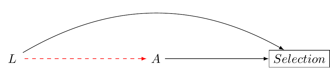
4. Collider bias and conditioning: Understanding how conditioning on colliders can induce bias in causal estimates, and how to avoid this issue.
5. Mediation and direct/indirect effects: if we are interested in total effects, we should not condition on a mediator.

Clear Advice for Drawing Causal Graphs

• Ensure that causes come before effects. Assign time indices to your variables.
• Organize your variables chronologically.
• Simplify your graph by removing unnecessary nodes that don’t impact the assessment of bias between an exposure and an outcome.
• Keep in mind that Directed Acyclic Graphs (DAGs) are qualitative tools. They don’t represent non-linear associations or interactions.
• Avoid depicting interactions by crossing arrows.
• Remember that DAGs are distinct from graphs used in Structural Equation Modeling (SEM). Be cautious of SEM literature, as it often overlooks the assumptions needed for causal inference.

Summary: Drawing Causal Graphs (DAGs)

• Directed Acyclic Graphs (DAGs) help visualize sources of bias.

• There are five main sources of bias:

  1. Temporal order ambiguity: Uncertainty about whether causes precede effects. Solution: Collect time series data or clarify assumptions when unavailable.
  2. Common causes of exposure and outcome: Address this by including common causes in your statistical model (e.g., using regression).
  3. Conditioning on a mediator: Avoid this unless mediation is of interest.
  4. Conditioning on a collider: Refrain from doing this.
  5. Bias induced by conditioning on a confounder’s descendant: Draw your DAG and follow guidelines for points 1-4.

• Important Note 1: In observational studies, it’s impossible to guarantee complete control for confounding. Always conduct sensitivity analyses. Techniques for sensitivity analyses will be discussed next week.

• Important Note 2: Methods for computing causal effects for group comparisons will be covered in the following week’s lecture.

Conclusion

In this lecture, we discussed the fundamental problem of causal inference, its assumptions, the role of randomized experiments in estimating causal effects, the challenges in identifying causal effects from observational data, and the use of causal graphs to represent and analyze causal relationships. You have learned how to use causal graphs to identify sources of bias. In the weeks ahead, we will apply this knowledge to address questions in cross-cultural psychology.

Reuse