---
title: "Self-Inflicted Injuries in Causal Inference"
subtitle: "Common Errors in Observational Studies"
author:
- name: Joseph A. Bulbulia
affiliation: Victoria University of Wellington, New Zealand
orcid: 0000-0002-5861-2056
email: joseph.bulbulia@vuw.ac.nz
date: 2025-08-12
editor_options:
chunk_output_type: console
---
```{r}
#| label: load_libraries
#| echo: false
#| include: false
#| eval: true
# load required libraries
library(tidyverse)
library(ggplot2)
library(patchwork)
library(gtsummary)
library(broom.helpers)
library(performance)
library(kableExtra)
# set theme for plots
theme_set(theme_minimal())
knitr::opts_chunk$set(
fig.width=9,
fig.asp = 0.5625,
out.width = "0.9\\linewidth",
fig.align = "center",
dpi = 300
)
```
# **Part 1: Motivating Example**
## 1990s observational studies indicated 30% all-cause mortality reduction from estrogen therapies?
::: {.callout-note title="In the 1980s and 1990s estrogen treatments appeared to **benefit** postmenopausal women"}
Hazard ratio for all-cause mortality: **0.68** current users vs. never users
[@grodstein2006hormone]
:::
## Standard Medical Advice
::: nonincremental
- 1992 American College of Obstetricians and Gynecologists \textcolor{cyan}{"Probable beneficial effect of estrogens on heart disease."}
- 1992 American College of Physicians \textcolor{cyan}{"Women who have coronary heart disease or who are at increased risk of coronary heart disease are likely to benefit from hormone therapy."}
- 1993 National Cholesterol Education Program \textcolor{cyan}{"Epidemiologic evidence for the benefit of estrogen replacement therapy is especially strong for secondary prevention in women with prior CHD."}
- 1996 American Heart Association \textcolor{cyan}{"ERT does look promising as a long-term protection against heart attack."}
:::
## Women's Health Initiative: Evaluate Estrogens Experimentally
::: nonincremental
- Massive **randomised**, double-blind, placebo-controlled trial
- 16,000 U.S. women aged 50-79 years
- Assigned to Estrogen plus Progestin therapy
- Women followed approximately every year for up to 8 years.
:::
## Findings: **Clear Discrepancy**
::: {.callout-warning title="Experimental Findings: **opposite of observational findings**" icon="false"}
All-cause mortality Hazard Ratio: **1.23** for initiators vs non-initiators. [@manson2003estrogen]
:::
## Medical community response: **Reject** all observational studies
::: nonincremental
- Can observational studies ever be trusted?
- Should observational studies ever be funded again?
- \color{cyan}{What went wrong?}
:::
## What is Causality?
## David Hume's Two Definitions in *Enquiries* (1751)
### Definition 1:
> We may define a cause to be an object followed by another, and where all the objects, similar to the first, are followed by objects similar to the second...
### Definition 2:
> Or, in other words, where, \color{cyan}{if the first object had not been, the second never would have existed}
*Enquiries Concerning Human Understanding, and Concerning the Principles of Morals* 1751
## Our lives are filled with "What If?" questions
*[Image: Sliding Doors movie poster - illustrating the "what if" concept]*
##
*[Image: Robert Frost poem - "Two roads diverged in a yellow wood"]*
## **The Fundamental Problem of Causal Inference**
To **quantify** a causal effect requires a **counterfactual** contrast:
$$\tau_{you} = \Big[Y_{\text{you}}(a =1) - Y_{\text{you}}(a=0)\Big]$$
Where, $Y(a)$ denotes the potential outcome under an intervention $A = a$. Here, we assume a binary intervention. At any time, we may observe the outcome of only \textcolor{red}{one intervention, not both.}
## However, we only observe *facts* not *counterfactuals*
$$
Y_i|A_i = 1 \implies Y_i(0)|A_i = 1~ \textcolor{red}{\text{is counterfactual}}
$$
::: footer
"**And sorry I could not travel both. And be one traveller, long I stood** $\dots$"
:::
## Average Treatment Effect in randomised controlled experiments work from assumptions
$$
\text{Average Treatment Effect} = \left[ \begin{aligned}
&\left( \underbrace{\mathbb{E}[Y(1)|A = 1]}_{\text{observed}} + \textcolor{cyan}{\underbrace{\mathbb{E}[Y(1)|A = 0]}_{\text{unobserved}}} \right) \\
&- \left( \underbrace{\mathbb{E}[Y(0)|A = 0]}_{\text{observed}} + \textcolor{cyan}{\underbrace{\mathbb{E}[Y(0)|A = 1]}_{\text{unobserved}}} \right)
\end{aligned} \right]
$$
## Under identifying assumptions, we may infer causal effects from associations
$$
\text{ATE} = \sum_{l} \left( \mathbb{E}[Y|A=1, \textcolor{cyan}{L=l}] - \mathbb{E}[Y|A=0, \textcolor{cyan}{L=l}] \right) \times \textcolor{cyan}{\Pr(L=l)}
$$
Where $L$ is a set of measured covariates and $A\coprod Y(a)|L$
# **Part 2: The First Self-Inflicted Error: The *What* Error**
## Paradigmatic Concern: Confounding by Common Cause
**[DAG: Common Cause]** - *A confounding variable L causes both treatment A and outcome Y*
## Where assumptions justify, we may condition on measured confounders to obtain balance.
::: {.panel-tabset}
## Problem
**[DAG: Common Cause]** - *A confounding variable L causes both treatment A and outcome Y*
## Solution
**[DAG: Adjusted for L]** - *By conditioning on L, we block the confounding path*
:::
# Error 1 – What (over-adjustment)
## "What Error #1": **Mediator Bias**
**[DAG: Mediator Bias]** - *Variable L mediates the effect of A on Y (A → L → Y)*
## Data Generating Process
```{r}
#| label: sim1-dgp
#| echo: true
#| eval: true
#| tbl-cap: "Religious Service (A) → Wealth (L) → Charity (Y). The true direct effect of A on Y is zero."
library(tidyverse)

set.seed(123)                           # reproducibility
n        <- 1000
service  <- rbinom(n, 1, 0.5)          # A
wealth   <- 2 * service + rnorm(n)     # L
charity  <- 1.5 * wealth + rnorm(n, sd = 1.5)  # Y

sim1 <- tibble(service, wealth, charity)
```
## Model comparison
```{r}
#| label: sim1-table
#| echo: false
#| message: false
#| warning: false
#| tbl-cap: "Controlling for the mediator reverses the sign of the service coefficient."
library(gtsummary)
library(broom.helpers)
fit_omit <- lm(charity ~ service, data = sim1) # correct
fit_adjust <- lm(charity ~ service + wealth, data = sim1) # biased
tbl_merge(
list(tbl_regression(fit_omit),
tbl_regression(fit_adjust)),
tab_spanner = c("Model A: Omit L",
"Model B: Control for L")
)
```
## Which model looks better?
```{r}
#| label: sim1-metrics
#| echo: true
#| eval: true
#| tbl-cap: "Model B wins on BIC and R² – yet its causal estimate is wrong."
library(performance)

compare_performance(fit_adjust, fit_omit, rank = TRUE)
# BIC(fit_adjust) - BIC(fit_omit) # negative → "better" fit
```
## "What Error #2": Collider Bias
**[DAG: Collider Bias]** - *Variable L is caused by both A and Y (A → L ← Y)*
## Data Generating Process
```{r}
#| label: sim2-dgp
#| echo: true
#| eval: true
#| tbl-cap: "Religious service (A) ← wealth (L) → donations (Y). A and Y are _independent_ in truth."
set.seed(2025)

n          <- 1000
service    <- rbinom(n, 1, 0.5)                            # A
donations  <- rnorm(n)                                     # Y
wealth     <- rnorm(n, mean = service + donations, sd = 1) # collider L

sim2 <- tibble(service, wealth, donations)
```
## Model Comparison
```{r}
#| label: sim2-table
#| echo: false
#| tbl-cap: "Adding the collider creates a spurious, significant effect of A."
fit_correct <- lm(donations ~ service, data = sim2) # correct
fit_biased <- lm(donations ~ service + wealth, data = sim2) # biased
tbl_merge(
list(tbl_regression(fit_correct),
tbl_regression(fit_biased)),
tab_spanner = c("Model A: Omit L",
"Model B: Control for L (collider)")
)
```
## Which model looks better?
```{r}
#| label: sim2-metrics
#| echo: true
#| eval: true
compare_performance(fit_biased, fit_correct, rank = TRUE)
BIC(fit_biased) - BIC(fit_correct)
```
## Take-Home
::: callout-important
Relying on model fit perpetuates the *causality crisis* in psychology [@bulbulia2022].
Draw the DAG first; decide what belongs in the model before looking at numbers.
:::
## The What Error is widespread in **experimental** studies in the social sciences
- "Overall, we find that **46.7% of the experimental studies** published in APSR, AJPS, and JOP from 2012 to 2014 engaged in posttreatment conditioning (35 of 75 studies) ..."
- "About **1 in 4 drop cases or subset the data based on post-treatment criteria,** and **nearly a third include post-treatment variables as covariates**"
- "Most tellingly, **nearly 1 in 8 articles directly conditions on variables that the authors themselves show as being an outcome of the experiment** -- an unambiguous indicator of **a fundamental lack of understanding ... that conditioning on posttreatment variables can invalidate results from randomized experiments.**"
- "Empirically, then, the answer to the question of **whether the discipline already understands posttreatment bias is clear: It does not.**" [@montgomery2018]
## Mediator Bias control strategy: **Longitudinal Hygiene**
::: columns
::: {.column width="50%"}
$$
\mediatorT
$$
:::
::: {.column width="50%"}
$$
\commoncausesolvedT
$$
:::
:::
## How to Tame The What Error? **Hide your future**
Use Repeated Measures on the Same Individuals
## Collider bias control strategy: **Hide your future**
::: columns
::: {.column width="50%"}
$$\colliderT$$
:::
::: {.column width="50%"}
$$\commoncausesolvedT$$
:::
:::
## Collider bias by proxy control strategy: **Hide your future**
::: columns
::: {.column width="50%"}
$$\commoncausechildT$$
:::
::: {.column width="50%"}
$$\commoncausesolvedchildT$$
:::
:::
## Post-exposure collider bias control strategy: **Hide your future**
::: columns
::: {.column width="50%"}
$$\mediatorcolliderT$$
:::
::: {.column width="50%"}
$$\commoncausesolvedT$$
:::
:::
## Finally, our biggest worry: **Unmeasured Common Causes**
$$\downstreamT$$
## Unmeasured common cause strategy: **Hide your future**
::: columns
::: {.column width="50%"}
$$\downstreamT$$
:::
::: {.column width="50%"}
$$\commoncausesolvedT$$
:::
:::
And because \textcolor{cyan}{hope is not enough}, we should consistently report sensitivity analyses.
<!-- The E-value is the minimum strength of association, on the risk ratio scale, that an unmeasured confounder would need to have with both the treatment and the outcome, conditional on the measured covariates, to explain away treatment–outcome association. -->
## Are longitudinal data + sensitivity analysis enough?
::: columns
::: {.column width="50%"}
If the data we collect were like this: $$Y_{\text{time 0}} ~~...~~ A_{\text{time 1}}$$
:::
::: {.column width="50%"}
We should not be tempted to model this.
$$\ytoacrazyT$$
:::
:::
## Are longitudinal data + sensitivity analysis enough?
\textcolor{cyan}{Too obvious} this is wrong?
$$\ytoacrazyT$$
# Error 2: When (time-zero)
## **Longitudinal data** are **not** enough
Temporal ordering was \textcolor{cyan}{precisely the problem} with the observational hormone studies in the 80s/90s that modelled \textcolor{cyan}{longitudinal data}.
**How?**
## Researchers failed to emulate an experiment in their data (Target Trial)
- Women's Health Initiative: overall hazard ratio 1.23 (0.99, 1.53)
- Women's Health Initiative: when broken down by years to follow-up:
- 0-2 years 1.51 (1.06, 2.14)
- 2-5 years 1.31 (0.93, 1.83)
- 5 or more years **0.67 (0.41, 1.09)**
::: {.callout-note title="Survivor Bias." icon="false"}
The observational results can be \textcolor{cyan}{entirely explained by selection bias}
:::
::: {.callout-note title="Emulating a target trial with observational data recovers experimental effects." icon="false"}
Re-modelling \textcolor{cyan}{initiation into hormone therapy} recovers experimental findings [@hernan2016].
:::
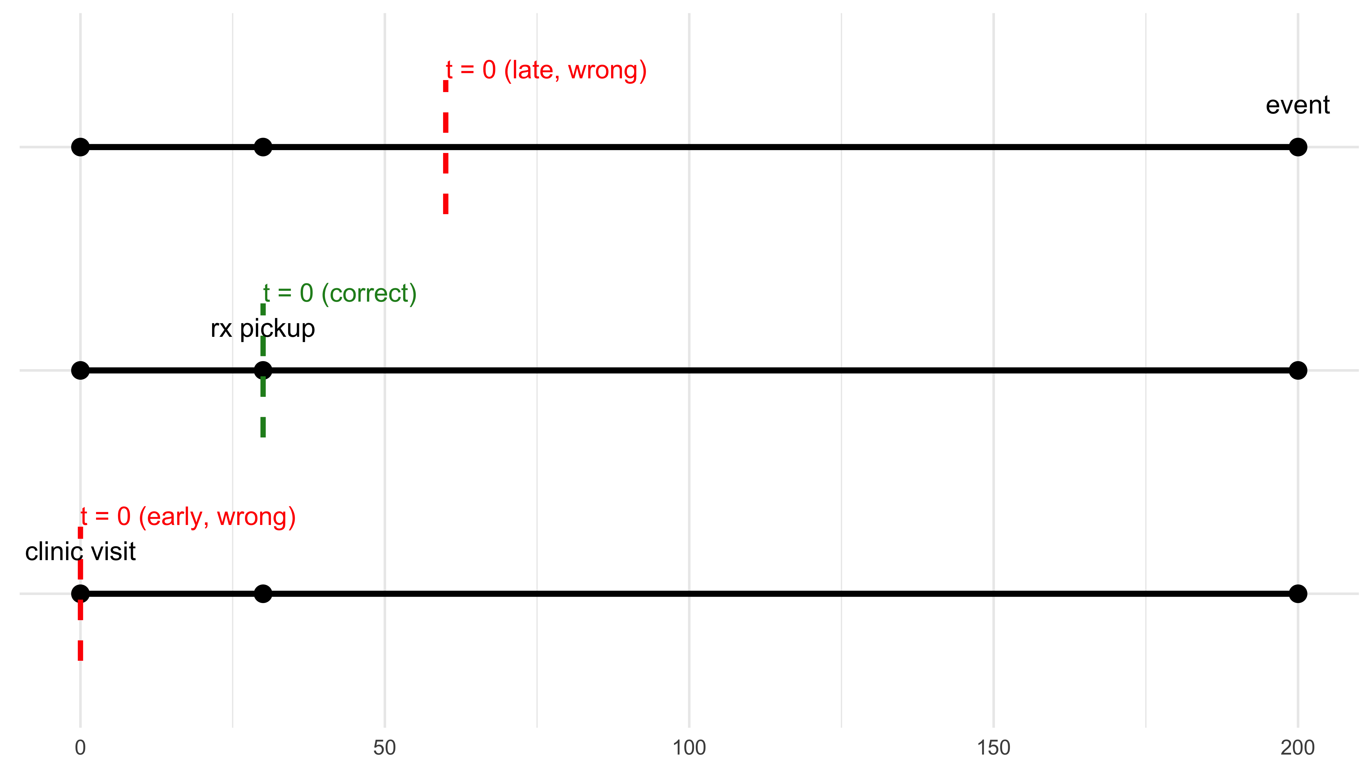
## Visualising the When Error
```{r}
#| label: fig-time-zero-3lines
#| fig-cap: "Three ways to start the clock. Only one is right."
#| fig-width: 8
#| fig-height: 4
#| echo: false
#| message: false
#| warning: false
library(tidyverse)
# lifeline coordinates ----------------------------------------------------
lifelines <- tibble(
scenario = factor(c("early time-zero", "correct time-zero", "late time-zero"),
levels = c("early time-zero", "correct time-zero", "late time-zero")),
clinic = 0, # day of clinic visit
rx = 30, # day prescription filled
event = 200 # day outcome occurs
)
# plot --------------------------------------------------------------------
ggplot(lifelines) +
## horizontal lifelines
geom_segment(aes(x = clinic, xend = event,
y = scenario, yend = scenario),
linewidth = 1.2) +
## milestone dots
geom_point(aes(x = clinic, y = scenario), size = 3) +
geom_point(aes(x = rx, y = scenario), size = 3) +
geom_point(aes(x = event, y = scenario), size = 3) +
## dashed t = 0 lines
# early (wrong)
geom_segment(x = 0, xend = 0, y = 0.7, yend = 1.3,
linetype = "dashed", colour = "red", linewidth = 1) +
# correct
geom_segment(x = 30, xend = 30, y = 1.7, yend = 2.3,
linetype = "dashed", colour = "forestgreen", linewidth = 1) +
# late (wrong)
geom_segment(x = 60, xend = 60, y = 2.7, yend = 3.3,
linetype = "dashed", colour = "red", linewidth = 1) +
## labels
annotate("text", x = 0, y = 1.35, label = "t = 0 (early, wrong)",
colour = "red", hjust = 0, size = 3.8) +
annotate("text", x = 30, y = 2.35, label = "t = 0 (correct)",
colour = "forestgreen", hjust = 0, size = 3.8) +
annotate("text", x = 60, y = 3.35, label = "t = 0 (late, wrong)",
colour = "red", hjust = 0, size = 3.8) +
annotate("text", x = 0, y = 1.05, label = "clinic visit", vjust = -1.2) +
annotate("text", x = 30, y = 2.05, label = "rx pickup", vjust = -1.2) +
annotate("text", x = 200, y = 3.05, label = "event", vjust = -1.2) +
theme_minimal() +
theme(axis.title = element_blank(),
axis.text.y = element_blank(),
axis.ticks = element_blank())
```
## Target Trial Check List
```{r}
#| label: tbl-target-trial
#| tbl-cap: "Target-trial specification for the hormone-therapy example."
#| echo: false
library(tidyverse)
library(kableExtra)
tribble(
~element, ~definition,
"Eligibility", "Post-menopausal women aged 50–79, no prior CHD",
"Treatment", "Initiate oestrogen + progestin on day of Rx pickup",
"Comparison", "No hormone-therapy initiation on that day",
"Outcome", "All-cause mortality",
"Follow-up", "8 years or until death / loss to follow-up"
) |>
kbl(booktabs = TRUE, align = "l") |>
kable_styling(latex_options = c("striped", "hold_position"))
```
# Error 3 – Who (population and heterogeneity)
## Illustration
# New Zealand Attitudes and Values Study (NZAVS): A step-by-step workflow for causal inference
## The New Zealand Attitudes and Values Study:
- Planned 20-year longitudinal study, currently in its 14th year, > 77k measured
- Sample frame is drawn randomly from the NZ Electoral Roll.
## Causal Questions
1) Average Treatment Effect: Difference in averages of social outcomes (a) if everyone in New Zealand were to attend religious service at least 1x per month (b) if everyone were not to attend religious service at all.
2) Heterogeneous Treatment Effects: Machine learning of groups who differ in such effects. Focus here on Qini Curve at 20% and 30% of full "budget".
3) Use Qini results to select for Policy Trees: Clarify *who* responds strongly/weakly.
**Note: all results use "honest" learning -- sample is split into training/test sets (here 70/30).**
## Outcomes
1. Sense of Belonging
2. Social Support
3. Charitable Donations (annual)
4. Volunteering (weekly)
**All outcomes measured one year after the intervention**
## Three-wave Panel Design: control for baseline exposure and outcome among confounder set.
$$
\threeLONG
$$
## Target Population: Residents of New Zealand in 2018 had they not been censored through 2021.
### Census Weights (Age X Gender X Ethnicity)

### (IPCW Stabilised & Trimmed)

## Religious Service Intervention
$$f(A) = \begin{cases} 1 & \text{if } a \ge 0 \text{ At least 1 x per month Religious Attendance} \\ 0 & \text{if } a = 0 \text{ Monthly Religious Service} \end{cases}$$
## Histogram Showing Split

## Love Plot of Propensity Scores

## Average Treatment Effect Results:
## Workflow
- Target population: New Zealand Population by 2018 census weights
- Outcomes: all NZAVS outcomes relating to pro-sociality (outcome-wide study)
- Missing data: inverse-probability of censoring weights non-parametrically estimated/ causal forests permit missing data at baseline
- Eligibility: participated in NZAVS 2018 (wave-10) and 2019 (wave 11, exposure wave) may have been lost to follow-up in wave 12, **46,377**.
- Bonferroni correct for multiple comparisons / E-value threshold = 1.2
## Transition table: Religious Attendance
|From / To | State 0| State 1| Total|
|:---------|-------:|-------:|-----:|
|State 0 | 28545| 681| 29226|
|State 1 | 887| 3593| 4480|
## Average Treatment Effect
The following outcomes showed reliable causal evidence (E‑value lower bound > 1.2):
- Volunteering (weekly, log): 0.154(0.056,0.252); on the original scale, 11.264 minutes(3.943,19.158). E‑value bound = 1.287
- log Charity Donate: 0.13(0.045,0.215); on the original scale, 39.935 (12.247,74.883). E‑value bound = 1.25
# Graph ATE

## How Much Better if We Treated by CATE?

## Who Should We Treat First? Belonging

## Who Should We Treat First? Charitable Donations

## Closing
| **Error** | **Need** | **Remedy** |
|-----------|----------------------------------|----------------------------------------------------|
| What | Control the right variables | Draw a DAG first |
| When | Start the clock on time | Emulate a target trial |
| Who | Treat the right people | Weight to target + investigate heterogeneity |
<!-- 3. Emulating experiments tend to \color{cyan}{attenuate results}. -->
## Thanks {.nonincremental}
::: nonincremental
- TRT Grant 0418 & Max Planck Institute for Evolutionary Anthropology for support.
- Chris G. Sibley (NZAVS lead Investigator) for the heavy data lifting
- 77,490 NZAVS participants for their time
- \textcolor{cyan}{Reach out} with questions or if you would like to become involved: \href{emailto:joseph.bulbulia@vuw.ac.nz}{joseph.bulbulia@vuw.ac.nz}
:::
------------------------------------------------------------------------

##
::: refs
:::