---
title: "Heterogeneity"
subtitle: "Moderation (as Effect Modification: Conditional Average Treatment Effects)"
date: "2025-NOV-19"
bibliography: /Users/joseph/GIT/templates/bib/references.bib
editor_options:
chunk_output_type: console
format:
html:
warnings: FALSE
error: FALSE
messages: FALSE
code-overflow: scroll
highlight-style: kate
code-tools:
source: true
toggle: FALSE
html-math-method: katex
cap-location: margin
---
```{=html}
<style>
.boxedblue {
border: 2px solid blue;
border-radius: 4px; /* slight roundness */
padding: 3px 6px; /* vertical | horizontal */
display: inline-block;
color: blue;
}
.circleblue {
border: 2px dashed blue;
border-radius: 50%;
padding: 3px 6px;
display: inline-block;
color: blue;
}
</style>
```
```{r setup, include=FALSE}
#| include: false
# libraries and functions (ensure these are accessible)
library("tinytex")
library(extrafont)
loadfonts(device = "win") # Adjust device based on OS if using extrafont
source("/Users/joseph/GIT/templates/functions/funs.R")
```
::: {.callout-note}
**Required Reading**
- [@hernan2024WHATIF] Chapters 4-5 [link](https://www.dropbox.com/scl/fi/9hy6xw1g1o4yz94ip8cvd/hernanrobins_WhatIf_2jan24.pdf?rlkey=8eaw6lqhmes7ddepuriwk5xk9&dl=0)
**Optional Reading**
- [@vanderweele2007FOURTYPESOFEFFECT] [link](https://www.dropbox.com/scl/fi/drytp2ui2b8o9jplh4bm9/four_types_of_effect_modification__a.6.pdf?rlkey=mb9nl599v93m6kyyo69iv5nz1&dl=0)
- [@vanderweele2009distinction] [link](https://www.dropbox.com/scl/fi/srpynr0dvjcndveplcydn/OutcomeWide_StatisticalScience.pdf?rlkey=h4fv32oyjegdfl3jq9u1fifc3&dl=0)
:::
::: {.callout-important}
**Key concepts**
- Causal estimand: The specific causal quantity of interest (e.g., the average effect in the population).
- Statistical estimand: The quantity computed from data to approximate the causal estimand.
- Interaction: The joint effect of two or more interventions.
- Effect modification: When the effect of one intervention varies by baseline characteristics.
- Heterogeneous treatment effects (HTE): The phenomenon that effects differ across individuals.
- Conditional average treatment effect (CATE), $\tau(x)$: The average effect for a subgroup with characteristics $x$.
- Estimated CATE, $\hat{\tau}(X)$: The empirical estimate of $\tau(x)$ for a subgroup defined by $X$.
:::
### The fundamental problem of causal inference
Consider whether bilingualism improves cognitive ability:
• $Y_i^{a=1}$: Cognitive ability of child $i$ if bilingual.
• $Y_i^{a=0}$: Cognitive ability of child $i$ if monolingual.
The individual causal effect is:
$$
Y_i^{a=1} - Y_i^{a=0}.
$$
If this difference $\neq 0$, bilingualism has an effect for $i$.
However, we observe only one potential outcome per child—physics prevents observing both.
Although individual effects are unobservable, average treatment effects (ATE) can be identified under assumptions:
$$
E(\delta) = E(Y^{a=1} - Y^{a=0}) = E(Y^{a=1}) - E(Y^{a=0}).
$$
### Identification assumptions**
#### Causal consistency:
The exposure levels compared correspond to well-defined interventions represented in the data.
### Positivity:
Every exposure level occurs with positive probability in all covariate strata.
### Exchangeability:
Conditional on measured covariates, exposure assignment is independent of potential outcomes.
We also assume::
#### Measurement error
Variables used to define exposures, outcomes, and confounders are measured without error or with error that does not induce bias after adjustment. Systematic or differential measurement error—especially in exposures or confounders—can bias effect estimates even when other assumptions hold.
#### Selection bias
The study sample is representative of the target population with respect to the causal effect of interest, or differences are accounted for through design or analysis. In longitudinal settings, attrition or loss to follow-up must not depend jointly on treatment and outcome in ways not captured by measured covariates; otherwise, the estimated effect may differ systematically from the true population effect.
#### Correctly Specified Model
This assumption is probably always violated in standard regression models
### Basic counterfactual logic
**Causal inference asks: What would happen under alternative interventions?**
For example, test scores $Y$ under:
- $a$: old teaching method,
- $a^*$: new teaching method.
The ATE:
$$
\mathbb{E}[Y(a^*) - Y(a)]
$$
is the average change in scores if the whole population switched from $a$ to $a^*$.
Confounding—common causes of $A$ and $Y$—must be addressed for valid inference.
### Interaction vs. effect modification
Interaction: Joint effects of two or more interventions.
Effect modification: Variation in the effect of a single intervention across subgroups.
#### Interaction
Let $A$ = teaching method, $B$ = tutoring, $Y$ = test score.
We compare:
- Effect of both: $\mathbb{E}[Y(1,1)] - \mathbb{E}[Y(0,0)]$
- Sum of individual effects: $\big(\mathbb{E}[Y(1,0)] - \mathbb{E}[Y(0,0)]\big) + \big(\mathbb{E}[Y(0,1)] - \mathbb{E}[Y(0,0)]\big)$.
#### Additive interaction exists if:
$$
\mathbb{E}[Y(1,1)] - \mathbb{E}[Y(1,0)] - \mathbb{E}[Y(0,1)] + \mathbb{E}[Y(0,0)] \neq 0.
$$
Positive values indicate synergy; negative values, antagonism.
Identification requires controlling for all confounders of $A \to Y$ ($L$) and $B \to Y$ ($Q$), i.e., $L \coprod Q$.
#### Effect modification and $\tau(x)$
Effect modification examines whether the effect of a single intervention $A$ on $Y$ differs by baseline characteristics $X$.
The conditional average treatment effect (CATE) is:
$$
\tau(x) = \mathbb{E}[Y(1) - Y(0) \mid X = x],
$$
the average effect for the subgroup with $X = x$.
Comparing $\tau(x)$ across $x$ quantifies effect modification.
If $X$ is categorical ($G$ = sex), group-specific ATEs are:
$$
\delta_{g} = \mathbb{E}[Y(1) \mid G=g] - \mathbb{E}[Y(0) \mid G=g],
$$
and effect modification exists if $\delta_{g_1} - \delta_{g_2} \neq 0$.
Identification requires adjusting for $A \to Y$ confounders within each group.
### Why psychology keeps confusing interactions with effect modification
Psychological papers typically fit linear models with multiplicative terms (e.g., `Y ~ A * M`) and call the coefficient on `A:M` “the interaction”. That coefficient is:
$$
\beta_{AM} = \frac{\partial^2 \mathbb{E}[Y \mid A, M]}{\partial A \, \partial M}
$$
It captures how the *statistical mean function* bends when we move both $A$ and $M$. This is useful for prediction, but it **is not** automatically an effect modifier because:
1. The cross-term blends confounding, scaling, and model misspecification. Unless the model is correctly specified and all confounders are solved, $\beta_{AM}$ has no causal meaning.
2. Even with perfect specification, $\beta_{AM}$ is a property of the *conditional mean*, not of potential outcome contrasts like $Y(1)-Y(0)$.
3. Psychologists often interact treatment with post-treatment mediators, which cannot identify effect modification because the mediator is itself altered by $A$.
Effect modification is about contrasts of potential outcomes stratified (or smoothed) over baseline features $X$; it is a *causal estimand*. Interactions in a single regression equation rarely align with that estimand.
**Rule of thumb**
> If you cannot write your estimand as $\mathbb{E}[Y(1)-Y(0)\mid X]$ for baseline $X$, you are not estimating a CATE. You're fitting a predictive surface with interaction terms.
### Causal forests pivot directly to $\tau(x)$
Generalised random forests (the `grf` package) estimate $\tau(x)$ without ever fitting a single interaction coefficient. Instead they:
1. Build trees that split on baseline covariates $X$ to expose treatment heterogeneity while enforcing honesty (separate subsamples for splits vs. estimation).
2. Average leaf-level treatment contrasts to produce $\hat{\tau}(x)$ for every unit.
3. Provide diagnostics (variance estimates, forest weights) so we can aggregate $\hat{\tau}(x)$ into interpretable summaries—RATE/Qini curves, policy trees, etc.
BIG implications:
- We no longer guess which pairwise interactions to include. The forest *discovers* the nonlinear combination of age and baseline charity in our simulation.
- $\hat{\tau}(x)$ respects causal identification (we still need consistency/positivity/exchangeability) but does not require a parametric regression form.
- CATE inference is local: we can report estimates (and uncertainty) for subgroups defined by the split structure rather than global $\beta_{AM}$ coefficients.
## HTE, CATE, and estimated $\hat{\tau}(x)$ in practice
- **HTE** means $\tau(x)$ is not constant; psychology often assumes it is.
- **CATE, $\tau(x)$** is the target: the average causal effect among units with baseline profile $x$.
- **Estimated CATE, $\hat{\tau}(x)$** is what `grf::causal_forest()` returns for each observation; we aggregate these to describe how effects vary.
For unit $i$ with profile $X_i=x$:
- The individual effect $Y_i(1)-Y_i(0)$ remains unobservable.
- $\hat{\tau}(x)$ is our best estimate of $\tau(x)$, derived from nearby observations that share $x$-like features in the forest’s learned metric.
Because $X$ is typically high-dimensional, manual interaction modeling is brittle. Causal forests—and the broader Margot workflow built around them—let us:
1. Estimate $\hat{\tau}(x)$ flexibly.
2. Diagnose whether detected heterogeneity is actionable (RATE/Qini, policy value).
3. Communicate effect modification in language policymakers understand (e.g., “Older, high-charity baseline participants benefit the most”).
This is the bridge between the theory of effect modification and the empirical machinery psychologists need to stop conflating statistical models results with causal moderation.
| Concept | Notation | Definition | Scope | Requirements |
|---------|----------|------------|-------|--------------|
| **Interaction** | – | Joint effect of multiple interventions compared with the sum of their separate effects | Multiple interventions ($A$, $B$) | Adjust for all confounders of $A \to Y$ and $B \to Y$ ($L \coprod Q$) |
| **Effect modification** | $\tau(x)$ varies with $x$ | Effect of a single intervention ($A$) differs by subgroup defined by $X = x$ | Single intervention | Adjust for confounders of $A \to Y$ within each subgroup |
| **Estimated CATE** | $\hat{\tau}(x)$ | Model-based estimate of $\tau(x)$ for $X = x$ | Prediction task | Flexible estimation methods (e.g., causal forests) |
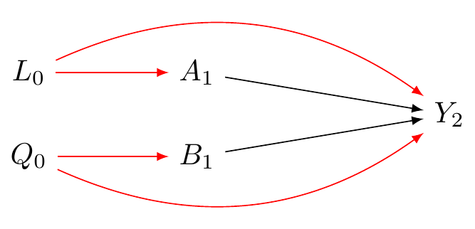
## Appendix: Identification of Interaction Effects
```{tikz}
#| label: fig-dag-interaction
#| fig-cap: "Diagram illustrating causal interaction. Assessing the joint effect of two interventions, A (e.g., teaching method) and B (e.g., tutoring), on outcome Y (e.g., test score). L represents confounders of the A-Y relationship, and Q represents confounders of the B-Y relationship. Red arrows indicate biasing backdoor paths requiring adjustment. Assumes A and B are decided independently here."
#| out-width: 100%
#| echo: false
\usetikzlibrary{positioning, shapes.geometric, arrows, decorations}
\tikzstyle{Arrow} = [->, thin, preaction = {decorate}]
\tikzset{>=latex}
\begin{tikzpicture}[{every node/.append style}=draw]
\node [rectangle, draw=white] (LA) at (0, .5) {$L_{0}$};
\node [rectangle, draw=white] (LB) at (0, -.5) {$Q_{0}$};
\node [rectangle, draw=white] (A) at (2, .5) {$A_{1}$};
\node [rectangle, draw=white] (B) at (2, -.5) {$B_{1}$};
\node [rectangle, draw=white] (Y) at (5, 0) {$Y_{2}$};
\draw [-latex, draw=red] (LA) to (A);
\draw [-latex, draw=red] (LB) to (B);
\draw [-latex, draw=red, bend left] (LA) to (Y);
\draw [-latex, draw=red, bend right] (LB) to (Y);
\draw [-latex, draw=black] (A) to (Y);
\draw [-latex, draw=black] (B) to (Y);
\end{tikzpicture}
```
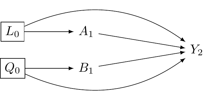
@fig-dag-interaction-solved shows we need to condition on (adjust for) *both* $L_0$ and $Q_0$.
```{tikz}
#| label: fig-dag-interaction-solved
#| fig-cap: "Identification of causal interaction requires adjusting for all confounders of A-Y (L) and B-Y (Q). Boxes around L and Q indicate conditioning, closing backdoor paths."
#| out-width: 80%
#| echo: false
\usetikzlibrary{positioning, shapes.geometric, arrows, decorations}
\tikzstyle{Arrow} = [->, thin, preaction = {decorate}]
\tikzset{>=latex}
\begin{tikzpicture}[{every node/.append style}=draw]
\node [rectangle, draw=black] (LA) at (0, .5) {$L_{0}$};
\node [rectangle, draw=black] (LB) at (0, -.5) {$Q_{0}$};
\node [rectangle, draw=white] (A) at (2, .5) {$A_{1}$};
\node [rectangle, draw=white] (B) at (2, -.5) {$B_{1}$};
\node [rectangle, draw=white] (Y) at (5, 0) {$Y_{2}$};
\draw [-latex, draw=black] (LA) to (A);
\draw [-latex, draw=black] (LB) to (B);
\draw [-latex, draw=black, bend left] (LA) to (Y);
\draw [-latex, draw=black, bend right] (LB) to (Y);
\draw [-latex, draw=black] (A) to (Y);
\draw [-latex, draw=black] (B) to (Y);
\end{tikzpicture}
```
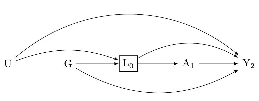
```{tikz}
#| label: fig-dag-effect-modification
#| fig-cap: "How shall we investigate effect modification of A on Y by G? Can you see the problem?"
#| out-width: 80%
#| echo: false
\usetikzlibrary{positioning, shapes.geometric, arrows.meta, decorations.pathmorphing}
\tikzset{
Arrow/.style={->, >=latex, line width=0.4pt}, % Defines a generic arrow style
emod/.style={rectangle, fill=blue!10, draw=blue, thick, minimum size=6mm},
emoddot/.style={circle, fill=blue!10, draw=blue, dotted, thick, minimum size=6mm}
}
\begin{tikzpicture}
\node [rectangle, draw=white, thick] (U) at (-4,0) {U};
\node [black] (G) at (-2,0) {G};
\node [rectangle, draw=black,thick] (L) at (0,0) {L$_{0}$};
\node [rectangle, draw=white, thick] (A) at (2,0) {A$_{1}$};
%\node [emoddot] (Z) at (0, -1) {Z};
\node [rectangle, draw=white, thick] (Y) at (4,0) {Y$_{2}$};
\draw[Arrow, draw=black, bend left = 20] (U) to (L);
\draw[Arrow, draw=black] (G) to (L);
\draw[Arrow, draw=black] (L) to (A);
\draw[Arrow, draw=black, bend left = 30] (L) to (Y);
\draw[Arrow, draw=black, bend right = 30] (G) to (Y);
\draw [-latex, draw=black] (A) to (Y);
\draw [-latex, draw=black,bend left = 40] (U) to (Y);
%\draw[-{Circle[open, fill=none]}, line width=0.25pt, draw=blue, bend right = 10] (Z) to (Y); % Circle-ended arrow
\end{tikzpicture}
```
Thus ,it is essential to understand that when we control for confounding along the the $A \to Y$ path, we do not identify the causal effects of effect-modifiers. Rather, we should consider effect-modifiers *prognostic* indicators. Moreover, we're going to need to develop methods for clarifying prognostic indicators in multi-dimensional settings where
<!-- ## Estimating How Effects Vary: Getting $\hat{\tau}(x)$ from Data -->
<!-- We defined the Conditional Average Treatment Effect (CATE), $\tau(x)$, as the *true* average effect for a subgroup with specific features $X=x$: -->
<!-- $$ -->
<!-- \tau(x) = \mathbb{E}[Y(1) - Y(0) | X = x] -->
<!-- $$ -->
<!-- Now, we want to *estimate* this from our actual data. We call our estimate $\hat{\tau}(x)$. For any person $i$ in our study with features $X_i$, the value $\hat{\tau}(X_i)$ is our data-based *prediction* of the average treatment effect *for people like person i*. -->
<!-- ### "Personalised" Effects vs. True Individual Effects -->
<!-- Wait - didn't we say we *can't* know the true effect for one specific person, $Y_i(1) - Y_i(0)$? Yes, that's still true. -->
<!-- So what does $\hat{\tau}(X_i)$ mean? -->
<!-- - **Individual Causal Effect (Unknowable):** $Y_i(1) - Y_i(0)$. This is the true effect for person $i$. We can't observe both $Y_i(1)$ and $Y_i(0)$. -->
<!-- - **Estimated CATE ($\hat{\tau}(X_i)$) (What we calculate):** This is our estimate of the *average* effect, $\mathbb{E}[Y(1) - Y(0)]$, for the *subgroup* of people who share the same measured characteristics $X_i$ as person $i$. -->
<!-- When people talk about "personalised" or "individualised" treatment effects in this context, they usually mean $\hat{\tau}(x)$. It's "personalised" because the prediction uses person $i$'s specific characteristics $X_i = x$. But remember, it's an **estimated average effect for a group**, not the unique effect for that single individual. -->
<!-- ### People Have Many Characteristics -->
<!-- People aren't just in one group; they have many features at once. A student might be: -->
<!-- - Female -->
<!-- - 21 years old -->
<!-- - From a low-income family -->
<!-- - Did well on previous tests -->
<!-- - Goes to a rural school -->
<!-- - Highly motivated -->
<!-- All these factors ($X_i$) together might influence how they respond to a new teaching method. -->
<!-- Trying to figure this out with traditional regression by manually adding interaction terms (like `A*gender*age*income*...`) becomes impossible very quickly: -->
<!-- - Too many combinations, not enough data in each specific combo. -->
<!-- - High risk of finding "effects" just by chance (false positives). -->
<!-- - Hard to know which interactions to even include. -->
<!-- - Can't easily discover unexpected patterns. -->
<!-- Thus, while simple linear regression with interaction terms (`lm(Y ~ A * X1 + A * X2)`) can estimate CATEs if the model is simple and correct, it often fails when things get complex (many $X$ variables, non-linear effects). -->
<!-- **Causal forests** (using the `grf` package in R) [@grf2024] are a powerful, flexible alternative designed for this task. They build decision trees that specifically aim to find groups with different treatment effects. -->
<!-- We'll learn how to use `grf` after the mid-term break. It will allow us to get the $\hat{\tau}(x)$ predictions and then think about how to use them, for instance, to prioritise who gets a treatment if resources are limited. -->
<!-- ### Summary -->
<!-- Let's revisit the centeral ideas: -->
<!-- #### **Interaction:** -->
<!-- - **Think:** Teamwork effect. -->
<!-- - **What:** Effect of *two or more different interventions* ($A$ and $B$) applied together. -->
<!-- - **Question:** Is the joint effect $\mathbb{E}[Y(a,b)]$ different from the sum of individual effects? -->
<!-- - **Needs:** Control confounders for *all* interventions involved ($L \coprod Q$). -->
<!-- #### **Effect Modification / HTE / CATE:** -->
<!-- - **Think:** Different effects for different groups. -->
<!-- - **What:** Effect of a *single intervention* ($A$) varies depending on people's *baseline characteristics* ($G$ or $X$). -->
<!-- - **Question (HTE):** *Does* the effect vary? (The phenomenon). -->
<!-- - **Question (CATE $\tau(x)$):** *What is* the average effect for a specific subgroup with features $X=x$? (The measure). -->
<!-- - **Needs:** Control confounders for the *single* intervention ($L$) within subgroups. -->
<!-- #### **Estimated "Individualised" Treatment Effects ($\hat{\tau}(x)$):** -->
<!-- - **Think:** Personal profile prediction, but for causal-effect **contrasts** -->
<!-- - **What:** Our *estimate* of the average treatment effect for the subgroup of people sharing characteristics $X_i$. -->
<!-- - **How:** Calculated using models (like causal forests) that use the person's full profile $X_i$. -->
<!-- - **Important:** This is **not** the true effect for that single person (which is unknowable). It's an average for *people like them*. -->
<!-- - **Use:** Explore HTE, identify subgroups, potentially inform targeted treatment strategies. -->
<!-- Keeping these concepts distinct helps us ask clear research questions and choose the right methods. -->
<!-- ## A Quick Recap -->
<!-- Let's quickly review the main ideas of causal inference we've covered. -->
<!-- ### The Big Question: Does A cause Y? -->
<!-- Causal inference helps us answer if something (like a teaching method, $A$) causes a change in something else (like test scores, $Y$). -->
<!-- ### Core Idea: "What If?" (Counterfactuals) -->
<!-- We compare what actually happened to what *would have happened* in a different scenario. -->
<!-- - $Y(1)$: Score if the student *had* received the new method. -->
<!-- - $Y(0)$: Score if the student *had* received the old method. -->
<!-- The **Average Treatment Effect (ATE)** = $\mathbb{E}[Y(1) - Y(0)]$ is the average difference across the whole group. -->
<!-- ### This Seminar Clarified Concepts of Interaction vs. Effect Modification vs. Individual Predictions -->
<!-- #### Interaction (Think: Teamwork Effects) -->
<!-- - **About:** Combining *two different interventions* (A and B). -->
<!-- - **Question:** Does using both A and B together give a result different from just adding up their separate effects? (e.g., new teaching method + tutoring). -->
<!-- - **Needs:** Analyse effects of A alone, B alone, and A+B together. Control confounders for *both* A and B. -->
<!-- #### Effect Modification (Think: Different Effects for Different Groups) -->
<!-- - **About:** How the effect of *one intervention* (A) changes based on people's *characteristics* (X, like prior grades). -->
<!-- - **Question:** Does the teaching method (A) work better for high-achieving students (X=high) than low-achieving students (X=low)? -->
<!-- - **HTE:** The *idea* that effects differ. -->
<!-- - **CATE $\tau(x)$:** The *average effect* for the specific group with characteristics $X=x$. -->
<!-- - **Needs:** Analyse effect of A *within* different groups (levels of X). Control confounders for A. -->
<!-- #### Estimated Individualised Effects ($\hat{\tau}(X_i)$) (Think: Personal Profile Prediction) -->
<!-- - **About:** Using a person's *whole profile* of characteristics ($X_i$ - age, gender, background, etc.) to predict their likely response to treatment A. -->
<!-- - **How:** Modern methods (like causal forests) take all of $X_i$ and estimate $\hat{\tau}(X_i)$. -->
<!-- - **Result:** this $\hat{\tau}(X_i)$ is **not** the true unknowable effect for person $i$. It is the estimated *average effect for people similar to person i* (sharing characteristics $X_i$). -->
<!-- - **Use:** helps explore if tailoring treatment based on these profiles ($X_i$) could be beneficial. -->
<!-- ### Summary: -->
<!-- - **Interaction:** Do A and B work together well/badly? -->
<!-- - **Effect Modification:** Does A's effect depend on *who* you are (based on X)? -->
<!-- - **$\hat{\tau}(X_i)$:** Can we *predict* A's average effect for someone based on their specific profile $X_i$? -->
<!-- Understanding these differences is key to doing good causal research! -->
<!-- ## Appendix: Simplification of Additive Interaction Formula -->
<!-- We start with the definition of additive interaction based on comparing the joint effect relative to baseline versus the sum of individual effects relative to baseline: -->
<!-- $$ -->
<!-- \Big(\mathbb{E}[Y(1,1)] - \mathbb{E}[Y(0,0)]\Big) - \Big[\Big(\mathbb{E}[Y(1,0)] - \mathbb{E}[Y(0,0)]\Big) + \Big(\mathbb{E}[Y(0,1)] - \mathbb{E}[Y(0,0)]\Big)\Big] -->
<!-- $$ -->
<!-- First, distribute the negative sign across the terms within the square brackets: -->
<!-- $$ -->
<!-- \mathbb{E}[Y(1,1)] - \mathbb{E}[Y(0,0)] - \Big(\mathbb{E}[Y(1,0)] - \mathbb{E}[Y(0,0)]\Big) - \Big(\mathbb{E}[Y(0,1)] - \mathbb{E}[Y(0,0)]\Big) -->
<!-- $$ -->
<!-- Now remove the parentheses, flipping the signs inside them where preceded by a minus sign: -->
<!-- $$ -->
<!-- \mathbb{E}[Y(1,1)] - \mathbb{E}[Y(0,0)] - \mathbb{E}[Y(1,0)] + \mathbb{E}[Y(0,0)] - \mathbb{E}[Y(0,1)] + \mathbb{E}[Y(0,0)] -->
<!-- $$ -->
<!-- Next, combine the $\mathbb{E}[Y(0,0)]$ terms: -->
<!-- * We have $2 x -\mathbb{E}[Y(0,0)]$ + -->
<!-- * 1x $+\mathbb{E}[Y(0,0)]$ -->
<!-- * leaving us with $+\mathbb{E}[Y(0,0)]$ -->
<!-- The expression simplifies -->
<!-- $$ -->
<!-- \mathbb{E}[Y(1,1)] - \mathbb{E}[Y(1,0)] - \mathbb{E}[Y(0,1)] + \mathbb{E}[Y(0,0)] -->
<!-- $$ -->
<!-- This is the standard definition of additive interaction. If this expression equals zero, there is no additive interaction; a negative value indicates a sub-attitive effect (antagonism), and positive value indicates an positive interaction (synergy). We have focussed on interaction on the difference scale, however, there are analagous estimands for ratio scales, see: [@vanderweele2009distinction; @bulbulia2024swigstime] -->
<!-- **This shows clearly that interaction is measured as the deviation of the joint effect from the sum of the separate effects, adjusted for the baseline.** -->
<!-- :::{.callout-note appearance="minimal"} -->
<!-- © 2025 Joseph Bulbulia. This work is licensed under a [Creative Commons Attribution-NonCommercial-ShareAlike 4.0 International License](https://creativecommons.org/licenses/by-nc-sa/4.0/). -->
<!-- ::: -->
## Group discussion
- Where in your field have 'interaction effects' been over-interpreted as causal moderation? Find an example and diagnose which assumption (baseline covariate, post-treatment mediator, model form) was actually violated.
- How would you explain to a collaborator the difference between $\beta_{AM}$ in a regression and $\tau(x)$ from a causal forest, without using equations: what metaphors would work in psychology?
- Suppose CATE estimates show that a subgroup benefits less. What ethical or practical considerations arise before recommending differentiated treatment, and how will you communicate that uncertainty?