Causal Inference: Average Treatment Effects
Suggested Readings - (Hernan and Robins 2020b) Chapters 1-3 link
- The Fundamental Problem of Causal Inference
- Causal Inference in Randomised Experiments
- Causal Inference in Observational Studies - Average (Marginal) Treatment Effects
- Three Fundamental Assumptions for Causal Inference
Here, we use the terms “counterfactual outcomes” and “potential outcomes” interchangeably.
Objectives
- You will understand why causation is never directly observed.
- You will understand how experiments address this “causal gap.”
- You will understand how applying three principles from experimental research allows human scientists to close this “causal gap” when making inferences about a population as a whole — that is, inferences about “marginal effects.”
Part 1: Motivating Example
1990s observational studies indicated 30% all-cause mortality reduction from estrogen therapies?
Standard Medical Advice
1992 American College of Obstetricians and Gynecologists {“Probable beneficial effect of estrogens on heart disease.”}
1992 American College of Physicians “Women who have coronary heart disease or who are at increased risk of coronary heart disease are likely to benefit from hormone therapy.”}
1993 National Cholesterol Education Program {“Epidemiologic evidence for the benefit of estrogen replacement therapy is especially strong for secondary prevention in women with prior CHD.”}
1996 American Heart Association {“ERT does look promising as a long-term protection against heart attack.”}
Women’s Health Initiative: Evaluate Estrogens Experimentally
Massive randomised, double-blind, placebo-controlled trial
16,000 U.S. women aged 50-79 years
Assigned to Estrogen plus Progestin therapy
Women followed approximately every year for up to 8 years.
Findings: Clear Discrepancy
Medical community response: Reject all observational studies
- Can observational studies ever be trusted?
- Should observational studies ever be funded again?
- {What went wrong?}
Opening
Robert Frost writes:
Two roads diverged in a yellow wood, And sorry I could not travel both And be one traveler, long I stood And looked down one as far as I could To where it bent in the undergrowth;
Then took the other, as just as fair, And having perhaps the better claim, Because it was grassy and wanted wear; Though as for that the passing there Had worn them really about the same,
And both that morning equally lay In leaves no step had trodden black. Oh, I kept the first for another day! Yet knowing how way leads on to way, I doubted if I should ever come back.
I shall be telling this with a sigh Somewhere ages and ages hence: Two roads diverged in a wood, and I— I took the one less traveled by, And that has made all the difference.
– The Road Not Taken
Introduction: Motivating Example
Consider the following question:
Alice attends religious service regularly. Does this increase her volunteering?
There is evidence that people who attend religious volunteer more, but would Alice volunteer anyway?
“And sorry I could not travel both. And be one traveler \dots”
Part 1: The Fundamental Problem of Causal Inference as a Missing Data Problem
The fundamental problem of causal inference is that causality is never directly observed.
Let Y an’a’d A denote random variables.
We formulate a causal question by asking whether experiencing a exposure A, when this exposure is set to level A = a, would lead to a difference in Y, compared to what would have occurred had the exposure been set to a different level, say A=a' will lead to a difference in outcome Y. For simplicity, we imagine binary exposure such that A = 1 denotes receiving the “religious service” exposure and A = 0 denotes receiving the “no religious service” exposure. Assume these are the only two exposures of interest:
Let:
- Y_i(a = 1) denotes Alice’s volunteering if Alice attended religious service (potential outcome when A_i = 1).
- Y_i(a = 0) denotes Alice’s volunteering if Alice did not attend religious service (potential outcome when A_i = 0).
What does it mean to quantify a causal effect.
We may define the individual-level causal effect of religious service on volunteering for a Alice (i) as the difference between two states of the world: one for which Alice experiences regular religious service and the other, not. We write this contrast by referring to the potential outcomes under different levels of exposure:
\text{Causal Effect}_i = Y_i(1) - Y_i(0).
We say there is a causal effect of religious service attendance if
Y_i(1) - Y_i(0) \neq 0.
Note, however – at most, only one of these two states can be observed.
Because each person experiences only one exposure condition in reality, we cannot directly compute this difference from any dataset — the missing observation is called the counterfactual:
- If Y_i|A_i = 1 is observed, then Y_i(0)|A_i=1 is counterfactual.
- If Y_i|A_i = 0 is observed, then Y_i(1)|A_i=1 is counterfactual.
Frost put it this way:
“And sorry I could not travel both / And be one traveler, long I stood \dots”
In short, individuals cannot simultaneously experience both exposure conditions, so we cannot quantitatively estimate individual-level causal effects (generally) because one outcome is inevitably missing.
How can we make contrasts between counterfactual (potential) outcomes?
Fundamental Assumption 1: Causal Consistency
Causal consistency means that the potential outcome corresponding to the exposure an individual actually receives is exactly what we observe. In other words, if individual i receives exposure a, then the potential outcome (or equivalently the counterfactual outcome under a given level of exposure A=a – that is Y_i(a) – is equivalent to the the observed outcome: Y_i \mid A_i \equiv a. Where the symbol \equiv means “equivalent to”, when we assume that the causal consistency assumption is satisfied, we assume that:
\begin{aligned} \underbrace{Y_i(1)}_{\text{counterfactual}} &\equiv \underbrace{(Y_i \mid A_i = 1)}_{\text{observable}}, \\ \underbrace{Y_i(0)}_{\text{counterfactual}} &\equiv \underbrace{(Y_i \mid A_i = 0)}_{\text{observable}}. \end{aligned}
Notice however that we cannot generally obtain individual causal effects because at any given time, each individual may only receive at most one leve of an exposure. Where the symbol \implies means “implies,” at any given time, receiving one level of an exposure precludes receiving any other level of that exposure:
Y_i|A_i = 1 \implies Y_i(0)|A_i = 1~ \text{is counterfactual} Likewise:
Y_i|A_i = 0 \implies Y_i(1)|A_i = 1~ \text{is counterfactual}
Because of the laws of physics (above the atomic scale), an individual can experience only one exposure level at any moment. Consequently, we can observe only one of the two counterfactual outcomes needed to quantify a causal effect. This is the fundamental problem of causal inference. Counterfactual contrasts cannot be individually observed.
However, because of the causal consistency assumption, we can nevertheless recover half of the missing counterfactual (or “potential”) outcomes needed to estimate average treatment effects. We may do this if two other assumptions are satisfied.
Fundamental Assumption 2: Exchangeability
Exchangeability justifies recovering unobserved counterfactuals from observed outcomes and averaging them. By accepting that Y_i(a) = Y_i if A_i = a, we can estimate population-level average potential outcomes. In an experiment where exposure groups are comparable, we define the Average Treatment Effect (ATE) as:
\begin{aligned} \text{ATE} &= \mathbb{E}[Y(1)] - \mathbb{E}[Y(0)] \\ &= \mathbb{E}(Y \mid A=1) \;-\; \mathbb{E}(Y \mid A=0). \end{aligned} Because randomisation (or more generally control over the probability of receiving treatment) ensures that missing counterfactuals are exchangeable with those observed, we can still estimate \mathbb{E}[Y(a)]. For instance, assume:
\underbrace{\mathbb{E}[Y(1)\mid A=1]}_{\text{counterfactual}} = \textcolor{red}{\underbrace{\mathbb{E}[Y(1)\mid A=0]}_{\text{unobservable}}} = \underbrace{(Y_i \mid A_i = 1)}_{\text{observed}}
which lets us infer the average outcome if everyone were treated. Likewise, if
\underbrace{\mathbb{E}[Y(0)\mid A=0]}_{\text{counterfactual}} = \textcolor{red}{\underbrace{\mathbb{E}[Y(1)\mid A=0]}_{\text{unobservable}}} = \underbrace{\mathbb{E}(Y \mid A_i = 0)}_{\text{observed}}
then we can infer the average outcome if everyone were given the control. The difference between these two quantities gives the ATE:
\text{ATE} = \Big[ \overbrace{\mathbb{E}[Y(1)\mid A=1]}^{\substack{\text{by consistency:}\\ \equiv \text{ observed } \; \mathbb{E}[Y\mid A=1]}} \;+\; \overbrace{\textcolor{red}{\mathbb{E}[Y(1)\mid A=0]}}^{\substack{\text{by exchangeability:}\\ \text{unobservable, yet } \; \equiv \mathbb{E}[Y\mid A=1]}} \Big] -\, \Big[ \overbrace{\mathbb{E}[Y(0)\mid A=0]}^{\substack{\text{by consistency:}\\ \equiv \text{observed } \; \mathbb{E}[Y\mid A=0]}} \;+\; \overbrace{\textcolor{red}{\mathbb{E}[Y(0)\mid A=1]}}^{\substack{\text{by exchangeability:}\\ \text{unobservable, yet } \; \equiv \mathbb{E}[Y\mid A=0]}} \Big]
We have it that \mathbb{E}[Y\mid A=1] and \mathbb{E}[Y\mid A=0] and \mathbb{E}[Y(1)\mid A=0] are observed. If both consistency and exchangeability are satisifed then we may use these observed quantities to identify contrasts of counterfactual quanities.
Thus, although individual-level counterfactuals are missing, the consistency assumptions and the exchangeability assumptions allow us to identify the average effect of treatment using observed data. Randomised controlled experiments allow us to meet these assumptions. Randomisation warrents the exchangeability assumption. Control warrents the consistency asumption.
Fundamental Assumption 3: Positivity
There is one further assumption, called positivity. It states that treatment assignments cannot be deterministic. That is, for every covariate pattern L = l, each individual has a non-zero probability of receiving ever treatment level to be compared:
P(A = a \mid L = l) > 0.
Randomised experiments achieve positivity by design – at least for the sample that is selected into the study. In observational settings violations occur if some subgroups never receive a particular treatment. If treatments occur but are rare, we may have sufficient data from which to obtain convincing causal inferences.
Positivity is the only assumption that can be verified with data.
Challenges with Observational Data
1. Satisfying Causal Consistency is Difficult in Observational Settings
Below are some ways in which real-world complexities can violate causal consistency in observational studies. For example, causal consistency requires there is no interference between units (also called “SUTVA” or “Stable Unit Treatment Value.” Causal consistency also requires that each treatment level is well-defined and applied uniformly. If these conditions fail, then Y(a) may not reflect a consistent exposures across individuals. We are then comparing apples with oranges. Consider some examples:
Cultural Dependence: one group’s “religious service” will differ qualitatively from another’s. Attending a !Kung! healing ritual and an Aztec human sacrifice may, plausible, produce different responses in people. In one, charity, in the other, terror.
Social Dependencies: Watts sees Alice gives, so Watts gives too. Here, effects under treatment differs depending on how others respond.
If the actual exposures differ across individuals, then consistency (Y_i(a) = Y_i \mid A_i) may fail, because A=a is not the same phenomenon for everyone.
2. Conditional Exchangeability (No Unmeasured Confounding) Is Difficult to Achieve
In theory, we can identify a causal effect from observational data if all confounders L are measured. Formally, we need the potential outcomes to be independent of treatment once we condition on L. One way to express this asssumption is: Y(a) \coprod A \mid L. If the potential outcomes are independent of treatment assignment, we can identify the Average Treatment Effect (ATE) as: \text{ATE} \;=\; \sum_{l} \Bigl[\mathbb{E}\bigl(Y \mid A=1, L=l\bigr) \;-\; \mathbb{E}\bigl(Y \mid A=0, L=l\bigr)\Bigr] \;\Pr(L=l).
In randomised experiments, conditioning is automatic because A is unrelated to potential outcomes by design. In observational studies, ensuring or approximating such conditional exchangeability is often difficult. For example, bilingualism research would need to consider:
- Cultural histories: cultures that value language acquistion might also value knowledge acquistion. Associations might arise from Culture, not causation.
- Personal values: families who place a high priority on bilingualism may also promote other developmental resources.
If important confounders go unmeasured or are poorly measured, these differences can bias causal effect estimates.
3. The Positivity Assumption May Fail: Treatments Might Not Exist for All
Positivity requires that each individual could, in principle, receive any exposure level. But in real-world observational settings, some groups have no access to bilingual education (or no reason to be monolingual), making certain treatment levels impossible for them. If a treatment level does not appear in the data for a given subgroup, any causal effect estimate for that subgroup is purely an extrapolation (Westreich and Cole 2010; Hernan and Robins 2020a).
Summary
We introduced the fundamental problem of causal inference by distinguishing correlation (associations in the data) from causation (contrasts between potential outcomes, of which only one can be observed for each individual).
Randomised experiments address this problem by balancing confounding variables across treatment levels. Although individual causal effects are unobservable, random assignment allows us to infer average causal effects — also called marginal effects.
In observational data, inferring average treatment effects demands that we satisfy three assumptions that are automatically satisfied in (well-conducted) experiments: causal consistency, exchangeability, and positivity. These assumptions ensure that we can compare like-with-like (that the population-level treatment effect is consistent across individuals), that there are no unmeasured common causes of the exposure and outcomes that may lead to associations in the absence of causality, and that every exposure level is a real possibility for each subgroup.
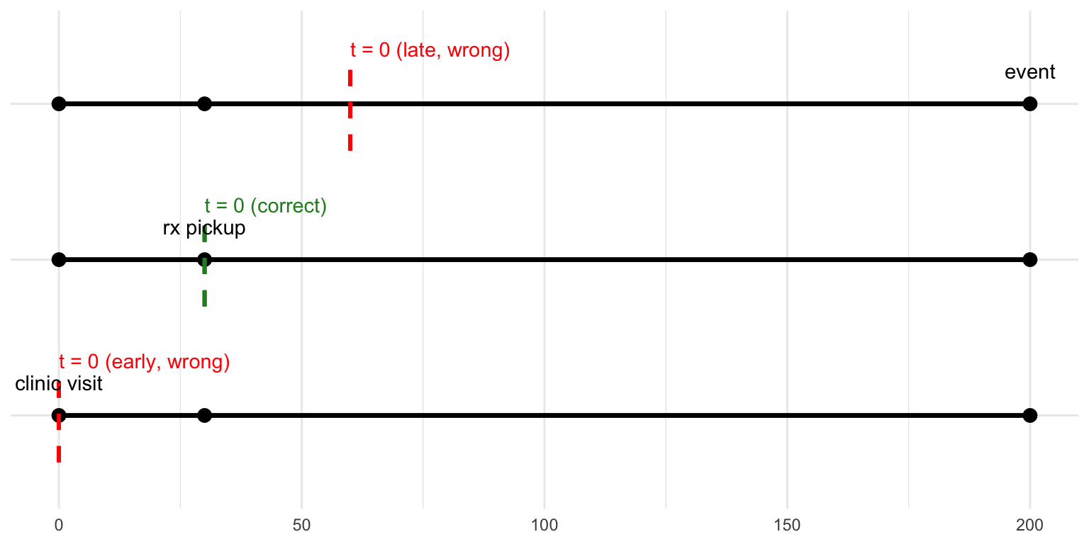
Motivating Example At The Start: The failure had nothing to do with causal assumptions but rather with setting up the data.
Longitudinal data are not enough: We must ask: when is TIME ZERO.
Temporal ordering was {precisely the problem} with the observational hormone studies in the 80s/90s that modelled .
How?
Researchers failed to emulate an experiment in their data (Target Trial)
Women’s Health Initiative: overall hazard ratio 1.23 (0.99, 1.53)
Women’s Health Initiative: when broken down by years to follow-up:
- 0-2 years 1.51 (1.06, 2.14)
- 2-5 years 1.31 (0.93, 1.83)
- 5 or more years 0.67 (0.41, 1.09)
Visualising the When Error
Key Take Home: Set Up Your Study Like an Experiment
| element | definition |
|---|---|
| Eligibility | Post-menopausal women aged 50–79, no prior CHD |
| Treatment | Initiate oestrogen + progestin on day of Rx pickup |
| Comparison | No hormone-therapy initiation on that day |
| Outcome | All-cause mortality |
| Follow-up | 8 years or until death / loss to follow-up |
–>
Group discussion
- Where in your own research program would an average treatment effect be the right estimand, and when would it hide disparities that stakeholders actually care about?
- Which of the three core identification assumptions (consistency, exchangeability, positivity) is most fragile in your field settings, and what concrete designs or measurements could shore it up?
- What are examples of post-treatment variables you have been tempted to adjust for, and how would doing so bias the total effect you are trying to interpret?
- Measurement error and selection bias were noted as “silent killers.” Share a case where either one flipped the sign or magnitude of an estimate, and outline how you’d redesign that study today.