---
title: "Causal inference: a step by step guide"
date: "2025-MAY-06"
bibliography: /Users/joseph/GIT/templates/bib/references.bib
editor_options:
chunk_output_type: console
format:
html:
warnings: FALSE
error: FALSE
messages: FALSE
code-overflow: scroll
highlight-style: Ayu
code-line-numbers: true
code-fold: true
code-tools:
source: true
toggle: false
html-math-method: katex
reference-location: margin
citation-location: margin
cap-location: margin
code-block-border-left: true
---
```{r}
#| include: false
#| echo: false
#read libraries
library("tinytex")
library(extrafont)
loadfonts(device = "all")
library("margot")
library("tidyverse")
```
::: {.callout-note}
**Required**
- grf package readings [https://grf-labs.github.io/grf/](https://grf-labs.github.io/grf/)
- Do "Homework" form Lecture 8
**Optional**
- [@Bulbulia2024PracticalGuide] [link](https://osf.io/preprints/psyarxiv/uyg3d)
- [@hoffman2023] [link](https://arxiv.org/pdf/2304.09460.pdf)
- [@vanderweele2020] [link](https://www.dropbox.com/scl/fi/srpynr0dvjcndveplcydn/OutcomeWide_StatisticalScience.pdf?rlkey=h4fv32oyjegdfl3jq9u1fifc3&dl=0)
:::
::: {.callout-important}
## Key concepts
Doing a causal analysis
:::
::: {.callout-important}
- Download the R script
- Download the relevant libraries.
- Will go through this script step-by-step.
:::
# Part 1: Laboratory
### Scripts for a full analysis
::: {.callout-note-script-0}
[Download full lab scripts 0](../laboratory/lab-10/00-setup-L10.R)
:::
::: {.callout-note-script-1}
[Download full lab scripts 1](../laboratory/ ../laboratory/lab-10/01-init-L10.R)
:::
::: {.callout-note-script-2}
[Download full lab scripts 2]( ../laboratory/lab-10/02-make-wide-L10.R)
:::
::: {.callout-note-script-3}
[Download full lab scripts 3](../laboratory/lab-10/03-models-L10-v3.R)
:::
## Script 0: Synthetic Data Fetch
**Run in full. No need to change anything.**
This script prepares your data. Run it once -- running it twice would be like turning the ignition off just to start your car again.
```{r}
#| include: true
#| eval: false
#| file: ../laboratory/lab-10/00-setup-L10.R
```
## Script 1: Initial Data Wrangling is HERE
```{r}
#| include: true
#| eval: false
#| file: ../laboratory/lab-10/01-init-L10.R
```
## Script 2: Make Wide Data Format With Censoring Weights is HERE
```{r}
#| include: true
#| eval: false
#| file: ../laboratory/lab-10/02-make-wide-L10.R
```
## Script 3: Models & Graphs is HERE
```{r}
#| include: true
#| eval: false
#| file: ../laboratory/lab-10/03-models-L10-v3.R
```
## Code Explanations
### Script 01 Initial Data Wrangling
Key checkpoints in the *wrangle-1* script are as follows;
#### First — pick your three study waves*
Note waves run from October --> September of the year following the wave.
Note:
- baseline variables must appear in the baseline wave
- the exposure variable must appear in both the baseline wave and exposure wave (but need not appear in the outcome wave)
- outcome variables must appear in both the baseline wave and outcome wave (but need not appear in the exposure wave.)
```r
# +--------------------------+
# |          ALERT           |
# +--------------------------+
# +--------------------------+
# | OPTIONALLY MODIFY SECTION|
# +--------------------------+

# **  define your study waves **
baseline_wave      <- "2018"        # baseline measurement
exposure_waves     <- c("2019")     # when exposure is measured
outcome_wave       <- "2020"        # when outcomes are measured
all_waves          <- c(baseline_wave, exposure_waves, outcome_wave)
```
#### Second — pick your exposure
Decide which variable is the 'cause'. Here it is `extraversion`. Verify it exists at baseline (`t0_`) *and* at the exposure wave (`t1_`)
```r
# define study variables ----------------------------------------------------
# ** key decision 2: define your exposure variable **

# +--------------------------+
# |          ALERT           |
# +--------------------------+
# +--------------------------+
# |    MODIFY THIS SECTION   |
# +--------------------------+
name_exposure <- "extraversion"

# exposure variable labels
var_labels_exposure <- list(
  "extraversion" = "Extraversion",
  "extraversion_binary" = "Extraversion (binary)"
)
# +--------------------------+
# |        END ALERT         |
# +--------------------------+
# +--------------------------+
# |   END MODIFY SECTION     |
# +--------------------------+
```
#### Third -- choose your outcome variables (ensuring they are in the baseline wave and outcome wave)
```r
# +--------------------------+
# |          ALERT           |
# +--------------------------+
# +--------------------------+
# |    MODIFY THIS SECTION   |
# +--------------------------+
# ** key decision 3: define outcome variables **
# here, we are focussing on a subset of wellbeing outcomes
# chose outcomes relevant to * your * study. Might be all/some/none/exactly
# these:
outcome_vars <- c(
  # health outcomes
  # "alcohol_frequency_weekly", "alcohol_intensity",
  # "hlth_bmi",
  "log_hours_exercise",
  # "hlth_sleep_hours",
  # "short_form_health",

  # psychological outcomes
  # "hlth_fatigue",
  "kessler_latent_anxiety",
  "kessler_latent_depression",
  "rumination",

  # well-being outcomes
  # "bodysat",
  #"forgiveness", "gratitude",
  "lifesat", "meaning_purpose", "meaning_sense",
  # "perfectionism",
  "pwi",
  #"self_control",
  "self_esteem",
  #"sexual_satisfaction",

  # social outcomes
  "belong", "neighbourhood_community", "support"
)
# +--------------------------+
# |   END MODIFY SECTION     |
# +--------------------------+
# +--------------------------+
# |        END ALERT         |
# +--------------------------+
```
#### Fourth: define baseline covariates
Define baseline variables. The primary role of these variables is to control unmeasured confounding. We will also use these variables to investigate treatment effect heterogeneity. Note that the exposure at baseline and the outcomes at baseline will automatically be included in this set later.
**You may use the following variables without modifying them.**
```r
# +--------------------------+
# |          ALERT           |
# +--------------------------+
# +--------------------------+
# | OPTIONALLY MODIFY SECTION|
# +--------------------------+
# define baseline variables -----------------------------------------------
# key decision 4 **  define baseline covariates **
# these are demographics, traits, etc. measured at baseline, that are common
# causes of the exposure and outcome.
# note we will automatically include baseline measures of the exposure and outcome
# later in the workflow.

baseline_vars <- c(
  # demographics
  "age", "born_nz_binary", "education_level_coarsen",
  "employed_binary", "eth_cat", "male_binary",
  "not_heterosexual_binary", "parent_binary", "partner_binary",
  "rural_gch_2018_l", "sample_frame_opt_in_binary",

  # personality traits (excluding exposure)
  "agreeableness", "conscientiousness", "neuroticism", "openness",

  # health and lifestyle
  "alcohol_frequency", "alcohol_intensity", "hlth_disability_binary",
  "log_hours_children", "log_hours_commute", "log_hours_exercise",
  "log_hours_housework", "log_household_inc",
  "short_form_health", "smoker_binary",

  # social and psychological
  "belong", "nz_dep2018", "nzsei_13_l",
  "political_conservative", "religion_identification_level"
)
# +--------------------------+
# |        END ALERT         |
# +--------------------------+
# +--------------------------+
# |   END MODIFY SECTION     |
# +--------------------------+
```
#### Five -- select baseline cohort population using eligibility criteria that are sensible for your study
```r
# +--------------------------+
# |          ALERT           |
# +--------------------------+
# +--------------------------+
# | OPTIONALLY MODIFY SECTION|
# +--------------------------+

# select eligible participants ----------------------------------------------
# only include participants who have exposure data at baseline

# You might require tighter conditions
# for example, if you are interested in the effects of hours of childcare,
# you might want to select only those who were parents at baseline.
# talk to me if you think you might night tighter eligibility criteria.

ids_baseline <- dat_prep |>
  # allow missing exposure at baseline
  # this would give us greater confidence that we generalise to the target population
  # filter(wave == baseline_wave) |>
  # option: do not allow missing exposure at baseline
  # this gives us greater confidence that we recover a incident effect
  filter(wave == baseline_wave, !is.na(!!sym(name_exposure))) |>
  pull(id)

# filter data to include only eligible participants and relevant waves
dat_long_1 <- dat_prep |>
  filter(id %in% ids_baseline, wave %in% all_waves) |>
  droplevels()

# +--------------------------+
# |END OPTIONALLY MODIFY SEC.|
# +--------------------------+
# +--------------------------+
# |        END ALERT         |
# +--------------------------+
```
#### Six -- choose a binary cut-point
Causal inference requires a contrast between two conditions. The splits give us the conditions of a hypothetical experiment.
```r
# +--------------------------+
# |          ALERT           |
# +--------------------------+
# +--------------------------+
# |    MODIFY THIS SECTION   |
# +--------------------------+
# define cutpoints
cut_points = c(1, 4)

# use later in positivity graph
lower_cut <- cut_points[[1]]
upper_cut <- cut_points[[2]]
threshold <- '>' # if upper

# save for manuscript
here_save(lower_cut, "lower_cut")
here_save(upper_cut, "upper_cut")
here_save(threshold, "threshold")

# make graph
graph_cut <- margot::margot_plot_categorical(
  dat_long_exposure,
  col_name         = name_exposure,
  sd_multipliers = c(-1, 1), # select to suit
  # either use n_divisions for equal-sized groups:
  # n_divisions      = 2,
  # or use custom_breaks for specific values:
  custom_breaks    = cut_points,  # ** adjust as needed **
  # could be "lower", no difference in this case, as no one == 4
  cutpoint_inclusive = "upper",
  show_mean        = TRUE,
  show_median      = FALSE,
  show_sd          = TRUE
)
print(graph_cut)

# save your graph
margot::here_save(graph_cut, "graph_cut", push_mods)
```
Ask: which break meaningfully separate groups into two exposure groups? Is the split *theoretically motivated**? adjust `custom_breaks` until the answer is 'yes'. then commit:
```r
dat_long_2 <- margot::create_ordered_variable(
  dat_long_1,
  var_name           = name_exposure,
  custom_breaks      = cut_points,  # ** -- adjust based on your decision above -- **
  cutpoint_inclusive = "upper"
)s
```
#### Seven — save as you go.
Use `margot::here_save()` (objects) and `here_save_qs()` (large objects) right after you create something you’ll cite in your report. The convention keeps analysis, tables, and manuscript in sync.
```r
here_save(dat_long_final,          "dat_long_final")
here_save(percent_missing_baseline,  "percent_missing_baseline")
```
#### Remember to check the positivity assumption
Is there change between `t0_` and `t1_` in the exposure variable?
```r
# create transition matrices to check positivity ----------------------------
# this helps assess whether there are sufficient observations in all exposure states
dt_positivity <- dat_long_final |>
  filter(wave %in% c(baseline_wave, exposure_waves)) |>
  select(!!sym(name_exposure), id, wave) |>
  mutate(exposure = round(as.numeric(!!sym(name_exposure)), 0)) |>
  # create binary exposure based on cutpoint
  mutate(exposure_binary = ifelse(exposure > upper_cut, 1, 0)) |> # check
  ## *-- modify this --*
  mutate(wave = as.numeric(wave) -1 )

# create transition tables
transition_tables <- margot::margot_transition_table(
  dt_positivity,
  state_var = "exposure",
  id_var = "id",
  waves = c(0, 1),
  wave_var = "wave",
  table_name = "transition_table"
)
print(transition_tables$tables[[1]])
margot::here_save(transition_tables, "transition_tables", push_mods)

# create binary transition tables
transition_tables_binary <- margot::margot_transition_table(
  dt_positivity,
  state_var = "exposure_binary",
  id_var = "id",
  waves = c(0, 1),
  wave_var = "wave",
  table_name = "transition_table_binary"
)
print(transition_tables_binary$tables[[1]])
margot::here_save(transition_tables_binary, "transition_tables_binary", push_mods)
```
#### Take-away: Think about the hypothetical experiment you wish to perform with observational data.
Decide early (exposure, cut-point, outcomes, waves), *checkpoint* everything with `here_save()`, and the rest of the pipeline flows.
### Script 2: Prepare Final Wide Data
**Purpose**
Convert the tidy long data into a grf-ready wide matrix and correct for dropout bias with inverse-probability-of-censoring weighting (IPCW).
#### Step 1 – go wide automatically
`margot_wide_machine()` reshapes each wave into `t0_`, `t1_`, `t2_` columns. You gave it all the names in script 1, so no new choices here. Inspect `df_wide` just to be sure the columns look sensible (baseline before exposure before outcome).
```r
colnames(df_wide)
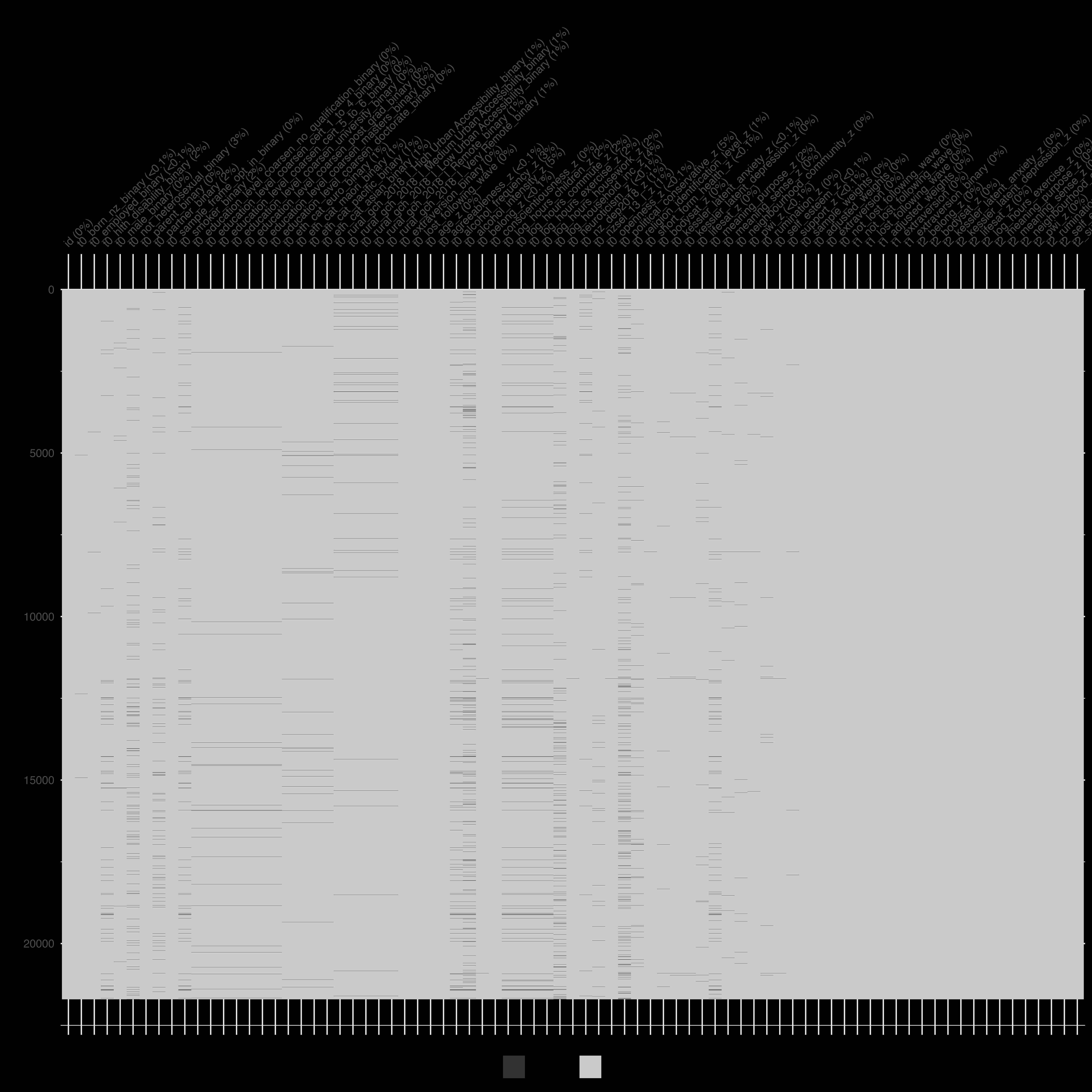
naniar::vis_miss(df_wide)
```
#### Step 2 – Encode + scale for algorithms
`margot_process_longitudinal_data_wider()` turns factors into dummies, scales continuous variables, and appends loss-to-follow-up flags. The result is `df_wide_encoded`.
Quick sanity check: the exposure binaries should be `0/1` and their `NA`s must match the *_lost* indicators.
```r
table(df_wide_encoded$t0_not_lost_following_wave)
```
#### Step 3 – Build IPCW weights*
**Why?** observations that resemble those who dropped out are up-weighted, so estimates stay unbiased when data vanish.
#### Step 4 – drop the censored
Rows with `*_lost_following_wave == 1` are removed, leaving `df_grf`. This dataset feeds the causal forest and should now have **no missing values** in any `t1_` or `t2_` column. Missingness is permitted in `t0_` columns
```r
naniar::vis_miss(df_grf)
```
{width=100%}
#### Step 5 – checkpoint everything
Each major object (`df_wide`, `df_wide_encoded`, `df_grf`, the weight vectors) is saved with `here_save()` or `here_save_qs()`. this keeps the analysis reproducible and the manuscript tables in sync.
#### Takeaway: what you must do
1. **Run the script without edits.**
2. confirm `df_grf` has the expected number of rows and no missing cells.
Script 2 is a conveyor belt: long $\to$ wide $\to$ weighted $\to$ clean. yYur only job is to eyeball the parcels before they roll into the modelling bay.
### Script 3 The Analysis
#### 1 Reproducibility scaffold
```r
set.seed(123)                 # lock randomness
pacman::p_load(margot, qs …)  # load every tool once
```
No choices here—just **run** and move on.
#### 2 Pull in prepared objects
```r
df_grf           <- here_read("df_grf")     # wide, weighted data
name_exposure    <- here_read("name_exposure")
```
If anything is `NULL`, return to scripts 1–2 and debug.
#### 3 Full model batches + ATE tables
Loop over the multiple outcome domains, saving each model to `models_example_2/`.
```r
models_binary <- margot_causal_forest(
  data = df_grf,
  outcome_vars = t2_outcome_z,
  covariates   = X, W = W, weights = weights,
  save_models  = TRUE, save_data = TRUE
)
here_save_qs(models_binary_health, "models_binary")
```
Then create ATE plots and interpretations with `margot_plot()`. Save as these go straight into the manuscript.
#### 4 Heterogeneous Treatment Effects (CATE)
- **Flip** outcomes you want to *minimise* (e.g. depression) so positive CATE = good. If your exposure is helpful, flip negative outcomes. If it is positive, flip positive outcomes.
```r
# flipping models: outcomes we want to minimise given the exposure --------
# standard negative outcomes/  not used in this example
# +--------------------------+
# |    MODIFY THIS           |
# +--------------------------+
flip_outcomes_standard = c(
  #"t2_alcohol_frequency_weekly_z",
  #"t2_alcohol_intensity_z",
  #"t2_hlth_bmi_z",
  #"t2_hlth_fatigue_z",
  "t2_kessler_latent_anxiety_z", #  ← select
  "t2_kessler_latent_depression_z",#  ← select
  "t2_rumination_z" #  ← select
  #"t2_perfectionism_z" # the exposure variable was not investigated
)

# when exposure is negative and you want to focus on how much worse off
# some people are use this:
# flip_outcomes<- c( setdiff(t2_outcomes_all, flip_outcomes_standard) )

# our example has the exposure as positive
flip_outcomes <- flip_outcomes_standard
```
Don't forget to get and save the labels for these models:
```r
# save
here_save(flip_outcomes, "flip_outcomes")


# get labels
flipped_names <- margot_get_labels(flip_outcomes, label_mapping_all)

# check
flipped_names

# save for publication
here_save(flipped_names, "flipped_names")


# this is a new function requires margot 1.0.48 or higher
label_mapping_all_flipped <- margot_reversed_labels(label_mapping_all, flip_outcomes)

# view
label_mapping_all_flipped

# save flipped labels # for any flipped results (reversed) is inserted in the label
here_save(label_mapping_all_flipped, "label_mapping_all_flipped")
```
Heterogenous Treatment Effect Workflow is as follows:
```r
# ──────────────────────────────────────────────────────────────────────────────
# SCRIPT:  HETEROGENEITY WORKFLOW
# PURPOSE: screen outcomes for heterogeneity, plot RATE & Qini curves,
#          fit shallow policy trees, and produce plain-language summaries.
# REQUIREMENTS:
#   • margot ≥ 1.0.52
#   • models_binary_flipped_all        – list returned by margot_causal_forest()
#   • original_df                      – raw data frame used in the forest
#   • label_mapping_all_flipped        – named vector of pretty labels
#   • flipped_names                    – vector of outcomes that were flipped
#   • decision_tree_defaults           – list of control parameters
#   • policy_tree_defaults             – list of control parameters
#   • push_mods                        – sub-folder for caches/outputs
#   • use 'models_binary', `label_mapping_all`, and set `flipped_names = ""` if no outcome flipped
# ──────────────────────────────────────────────────────────────────────────────

# check package version early
stopifnot(utils::packageVersion("margot") >= "1.0.52")

# helper: quick kable printer --------------------------------------------------
print_rate <- function(tbl) {
  tbl |>
    mutate(across(where(is.numeric), \(x) round(x, 2))) |>
    kbl(format = "markdown")
}

# 1  SCREEN FOR HETEROGENEITY (RATE AUTOC + RATE Qini)  ----------------------

rate_results <- margot_rate(
  models        = models_binary_flipped_all,
  policy        = "treat_best",
  alpha         = 0.20,        # keep raw p < .20
  adjust        = "fdr",       # false-discovery-rate correction
  label_mapping = label_mapping_all_flipped
)

print_rate(rate_results$rate_autoc)
print_rate(rate_results$rate_qini)
# convert RATE numbers into plain-language text
rate_interp <- margot_interpret_rate(
  rate_results,
  flipped_outcomes      = flipped_names,
  adjust_positives_only = TRUE
)

cat(rate_interp$comparison, "\n")
cli_h2("Analysis ready for Appendix ✔")

# organise model names by evidence strength
model_groups <- list(
  autoc       = rate_interp$autoc_model_names,
  qini        = rate_interp$qini_model_names,
  either      = rate_interp$either_model_names,
  exploratory = rate_interp$not_excluded_either
)

# 2  PLOT RATE AUTOC CURVES ---------------------------------------------------

autoc_plots <- margot_plot_rate_batch(
  models        = models_binary_flipped_all,
  save_plots    = FALSE,  # set TRUE to store .png files
  label_mapping = label_mapping_all_flipped,
  model_names   = model_groups$autoc
)

# inspect the first curve - note there may be more/none.
# if none, comment out
autoc_plots[[1]]
autoc_name_1 <- rate_results$rate_autoc$outcome[[1]]

# 3  QINI CURVES + GAIN INTERPRETATION ---------------------------------------
qini_results <- margot_policy(
  models_binary_flipped_all,
  save_plots         = FALSE,
  output_dir         = here::here(push_mods),
  decision_tree_args = decision_tree_args,
  policy_tree_args   = policy_tree_args,
  model_names        = names(models_binary_flipped_all$results),
  original_df        = original_df,
  label_mapping      = label_mapping_all_flipped,
  max_depth          = 2L,
  output_objects     = c("qini_plot", "diff_gain_summaries")
)

qini_gain <- margot_interpret_qini(
  qini_results,
  label_mapping = label_mapping_all_flipped
)

print_rate(qini_gain$summary_table)
cat(qini_gain$qini_explanation, "\n")

reliable_ids <- qini_gain$reliable_model_ids

# (re-)compute plots only for models that passed Qini reliability
qini_results_valid <- margot_policy(
  models_binary_flipped_all,
  save_plots         = FALSE,
  output_dir         = here::here(push_mods),
  decision_tree_args = decision_tree_args,
  policy_tree_args   = policy_tree_args,
  model_names        = reliable_ids,
  original_df        = original_df,
  label_mapping      = label_mapping_all_flipped,
  max_depth          = 2L,
  output_objects     = c("qini_plot", "diff_gain_summaries")
)

qini_plots <- map(qini_results_valid, ~ .x$qini_plot)

# grab pretty outcome names
qini_names <- margot_get_labels(reliable_ids, label_mapping_all_flipped)

cli_h1("Qini curves generated ✔")

# 4  POLICY TREES (max depth = 2) -------------------------------------------

policy_results_2L <- margot_policy(
  models_binary_flipped_all,
  save_plots         = FALSE,
  output_dir         = here::here(push_mods),
  decision_tree_args = decision_tree_defaults,
  policy_tree_args   = policy_tree_defaults,
  model_names        = reliable_ids,      # only those passing Qini
  max_depth          = 2L,
  original_df        = original_df,
  label_mapping      = label_mapping_all_flipped,
  output_objects     = c("combined_plot")
)

policy_plots <- map(policy_results_2L, ~ .x$combined_plot)

# ️5  PLAIN-LANGUAGE INTERPRETATION OF TREES ----------------------------------

policy_text <- margot_interpret_policy_batch(
  models            = models_binary_flipped_all,
  original_df       = original_df,
  model_names       = reliable_ids,
  label_mapping     = label_mapping_all_flipped,
  max_depth         = 2L
)

cat(policy_text, "\n")

cli::cli_h1("Finished: depth-2 policy trees analysed ✔")
```
#### 5 Report subgroup analyses (optional)
When theory predicts effect modification—age bands, income thirds, etc.—use `margot_planned_subgroups_batch()`.
Here's the workflow:
```r
# ------------------------------------------------------------------------------
# purpose: explores effect heterogeneity across researcher-defined strata (appendix only)
# ------------------------------------------------------------------------------
# workflow philosophy -----------------------------------------------------------
# • descriptive, not prescriptive. we *report* how τ̂ varies over groups – we do
#   NOT optimise a policy rule.
# • strata = ±1 sd splits by default; change to suit theory.
# • code chunks are short and labelled so students can run/debug in order.
# ------------------------------------------------------------------------------

library(margot)      # ≥ 1.0.52
library(tidyverse)   # pipes + helpers
library(knitr)       # kable tables
library(patchwork)   # plot stacks

# check package version early ---------------------------------------------------
stopifnot(utils::packageVersion("margot") >= "1.0.52")

# ------------------------- 1. define strata -----------------------------------
# 0. back‑transform helper -------------------------------------------
# margot stores income as z‑scored log dollars.  to write interpretable
# subtitles we convert ±1 sd back to the raw scale.  the helper simply
# inverts the: log → z transformation.
log_mean_inc <- mean(original_df$t0_log_household_inc, na.rm = TRUE)
log_sd_inc   <- sd  (original_df$t0_log_household_inc, na.rm = TRUE)

margot_back_transform_log_z(
  log_mean = log_mean_inc,
  log_sd   = log_sd_inc,
  z_scores = c(-1, 0, 1),
  label    = "data_scale"   # prints nz$ values ≈ 41k,…
)

# 1. define strata via logical vectors -------------------------------
# we treat ±1sd as the default cut for “low / mid / high”.  students
# can change the thresholds or supply any logical `subset_condition`.
complex_condition_political <- between(X[, "t0_political_conservative_z"], -1, 1)
complex_condition_wealth    <- between(X[, "t0_log_household_inc_z"], -1, 1)
complex_condition_age       <- between(X[, "t0_age_z"], -1, 1)

# sanity‑check age bounds on the raw scale
mean(original_df$t0_age) + c(-1, 1) * sd(original_df$t0_age)

# wealth -----------------------------------------------------------------------
subsets_standard_wealth <- list(
  Poor   = list(
    var = "t0_log_household_inc_z",
    value = -1,
    operator = "<",
    description = "income < −1sd (≈ NZ$41k)",
    label = "Poor"
  ),
  MiddleIncome = list(subset_condition = complex_condition_wealth, description = "income within ±1sd (≈ NZ$41‑191k)"),
  Rich   = list(
    var = "t0_log_household_inc_z",
    value = 1,
    operator = ">",
    description = "income > +1sd (≈ NZ$191k)",
    label = "Rich"
  )
)
# political orientation --------------------------------------------------------
subsets_standard_political <- list(
  Liberal = list(
    var = "t0_political_conservative_z",
    value = -1,
    operator = "<",
    description = "Effects among those < -1 SD in political conservativism",
    label = "Liberal"
  ),
  Centrist = list(
    var = "t0_political_conservative_z",
    # operator = "<",
    subset_condition = complex_condition_political,
    description = "Effects among those > -1 SD and < +1 in political conservativism",
    label = "Centrist"
  ),
  Conservative = list(
    var = "t0_political_conservative_z",
    value = 1,
    operator = ">",
    description = "Effects among those > +1 SD in political conservativism",
    label = "Conservative"
  )
)

# age --------------------------------------------------------------------------
subsets_standard_age <- list(
  Younger = list(
    var = "t0_age_z",
    value = -1,
    operator = "<",
    label = "Age < 35"
  ),
  Middle = list(
    var = "t0_age_z",
    # operator = "<",
    subset_condition = complex_condition_age,
    label = "Age 35-62"
  ),
  Older = list(
    var = "t0_age_z",
    value = 1,
    operator = ">",
    label = "Age > 62"
  )
)

# gender (binary) --------------------------------------------------------------
subsets_standard_gender <- list(
  Female = list(
    var = "t0_male_binary",
    value = 0,
    description = "Females"
  ),
  Male = list(
    var = "t0_male_binary",
    value = 1,
    description = "Males"
  )
)

# ethnicity (binary dummies) --------------------------------------------------
subsets_standard_ethnicity <- list(
  Asian = list(
    var = "t0_eth_cat_asian_binary",
    value = 1,
    label = "Asians",
    description = "Asians"

  ),
  Euro = list(
    var = "t0_eth_cat_euro_binary",
    value = 1,
    label = "NZ Europeans ",
    description = "NZ Europeans"

  ),
  Pacific = list(
    var = "t0_eth_cat_pacific_binary",
    value = 1,
    label = "Pacific Peoples",
    description =  "Pacific Peoples"
  ),
  Maori = list(
    var = "t0_eth_cat_maori_binary",
    value = 1,
    label = "Māori",
    description = 'Māori'
  )
)
# religion ---------------------------------------------------------------------
subsets_standard_secular_vs_religious <- list(
  Not_Religious = list(var = "t0_religion_bigger_denominations_not_rel_binary", value = 1, label = "Not Religious"),
  Religious = list(var = "t0_religion_bigger_denominations_not_rel_binary", value = 0, label = "Religious")
)

# ------------------------- 2. defaults for ATE plots --------------------------
# set up domain names
domain_names <- c("wellbeing")

# set up subtitles
subtitles <- ""

# play around with these values
x_offset_comp <- 1.0
x_lim_lo_comp <- -1.0
x_lim_hi_comp <- 1.0

base_defaults_comparisons <- list(
  type = "RD",
  title = ate_title,
  e_val_bound_threshold = 1.2,
  label_mapping = label_mapping_all,
  adjust = "bonferroni",
  #<- new
  alpha = 0.05,
  # <- new
  colors = c(
    "positive" = "#E69F00",
    "not reliable" = "grey50",
    "negative" = "#56B4E9"
  ),
  x_offset = x_offset_comp,
  # will be set based on type
  x_lim_lo = x_lim_lo_comp,
  # will be set based on type
  x_lim_hi = x_lim_hi_comp,
  text_size = 8,
  linewidth = 0.75,
  estimate_scale = 1,
  base_size = 18,
  point_size = 2.5,
  title_size = 19,
  subtitle_size = 16,
  legend_text_size = 10,
  legend_title_size = 10,
  include_coefficients = FALSE
)

# ------------------------- 3. batch subgroup analysis -------------------------
planned_subset_results <- margot_planned_subgroups_batch(
  domain_models = list(models_binary),
  X             = X,
  base_defaults = base_defaults,
  subset_types  = list(
    wealth              = subsets_wealth,
    political_orientation = subsets_political,
    age                 = subsets_age,
    gender              = subsets_gender,
    ethnicity           = subsets_ethnicity,
    religion            = subsets_religion
  ),
  original_df   = original_df,
  label_mapping = label_mapping_all,
  domain_names  = "wellbeing",
  adjust        = "bonferroni",
  alpha         = 0.05,
  subtitles  = subtitles
)

# ------------------------- 4. quick summaries ---------------------------------
cat(planned_subset_results$wellbeing$wealth$explanation)
cat(planned_subset_results$wellbeing$political_orientation$explanation)
cat(planned_subset_results$wellbeing$age$explanation)

# ------------------------- 5. example plots -----------------------------------
# wealth – vertical stack
wrap_plots(
  list(
    planned_subset_results$wellbeing$wealth$results$Poor$plot,
    planned_subset_results$wellbeing$wealth$results$`Middle Income`$plot,
    planned_subset_results$wellbeing$wealth$results$Rich$plot
  ),
  ncol = 1
) +
  plot_annotation(
    title = "Wealth",
    theme = theme(plot.title = element_text(size = 18, face = "bold"))
  )

# ethnicity – 2×2 grid
wrap_plots(
  list(
    planned_subset_results$wellbeing$ethnicity$results$Asian$plot,
    planned_subset_results$wellbeing$ethnicity$results$`NZ European`$plot,
    planned_subset_results$wellbeing$ethnicity$results$Pacific$plot,
    planned_subset_results$wellbeing$ethnicity$results$Māori$plot
  ),
  ncol = 2
) +
  plot_annotation(
    title = "Ethnicity",
    theme = theme(plot.title = element_text(size = 18, face = "bold"))
  )
```
Note, unless there are theoretical reasons to expect subgroup differences we should be *cautious* about inferring too much.
We can also compare groups to each other using code such as this, however we should only do so if there is theoretical motivation.
```r
# ------------------------- 6. group-vs-group example --------------------------
comp_age <- margot_compare_groups(
  group1_name    = "Under 35",
  group2_name    = "Over 62",
  planned_subset_results$wellbeing$age$results$`Age < 35`$transformed_table,
  planned_subset_results$wellbeing$age$results$`Age > 62`$transformed_table,
  type           = "RD",
  decimal_places = 3
)
print(comp_age$results |> kbl("markdown", digits = 2))
cat(comp_age$interpretation)

cli::cli_h1("subgroup analysis complete ✔")


# example: secular vs religious
group_comparison_secular_religious <- margot_compare_groups(
  group1_name = "Secular People",
  group2_name = "People Who Identify With Religion",
  planned_subset_results$wellbeing$religion$results$`Not Religious`$transformed_table,
  # reference
  planned_subset_results$wellbeing$religion$results$Religious$transformed_table,
  # reference
  type            = "RD",
  # risk‑difference scale
  decimal_places  = 3
)
print(group_comparison_secular_religious$results |> kbl("markdown", digits = 2))
cat(group_comparison_secular_religious$interpretation)
```
```r
# 6. group‑vs‑group comparisons --------------------------------------
#   • `margot_compare_groups()` takes two transformed tables (risk‑diff)
#   • returns a *difference in differences* tibble + plain‑text interp.

# example: young (<35) vs older (>62)
group_comparison_age_young_old <- margot_compare_groups(
  planned_subset_results$wellbeing$cohort$results$`Age < 35`$transformed_table, # reference
  planned_subset_results$wellbeing$cohort$results$`Age > 62`$transformed_table, # comparison
  type            = "RD",          # risk‑difference scale
  decimal_places  = 4
)
print(group_comparison_age_young_old$results |> kbl("markdown", digits = 2))
cat(group_comparison_age_young_old$interpretation)
```
#### Takeaway
Run the script in order, **eyes on three checkpoints**: the toy forest plot, convincing Qini/RATE curves/interpretations, and sensible policy-tree leaves. Everything else is auto-saved for the manuscript.
# Part 2:
- **Sensitivity Analysis: E-values**
- **Workflow**
<!-- ### Modified Treatment Policies and E-values -->
<!-- A modified treatment policy is a *flexible* intervention of the following form: -->
<!-- $$ -->
<!-- \mathbf{d}^\lambda (a_1) = \begin{cases} 4 & \text{if } a_1 < 4 \\ -->
<!-- a_1 & \text{otherwise} \end{cases} -->
<!-- $$ -->
<!-- $$ -->
<!-- \mathbf{d}^\phi (a_1) = \begin{cases} 0 & \text{if } a_1 > 0 \\ -->
<!-- a_1 & \text{otherwise} \end{cases} -->
<!-- $$ -->
<!-- $$ g' = \text{Intervention 1 - Intervention 2} = E[Y(\mathbf{d}^\lambda) - Y(\mathbf{d}^\phi)] $$ -->
<!-- $$ g'' = \text{Intervention 1 - Intervention 2} = E[Y(\mathbf{d}^\lambda) - Y(\mathbf{d}^\phi)] $$ -->
<!-- $$ -->
<!-- {\delta}(g) ={g'} - {g''} -->
<!-- $$ -->
<!-- Rather than shifting an entire population into one of two states, the estimand flexibly shifts a population according to a pre-specified function. -->
<!-- see: @hoffman2023 -->
### Sensitivity Analysis using E-values
> The minimum strength of association on the risk ratio scale that an unmeasured confounder would need to have with both the exposure and the outcome, conditional on the measured covariates, to fully explain away a specific exposure-outcome association
See: @mathur2018; @linden2020EVALUE; @vanderweele2017.
For example, suppose that the lower bound of the the E-value was 1.3 with the lower bound of the confidence interval = 1.12, we might then write:
> With an observed risk ratio of RR=1.3, an unmeasured confounder that was associated with both the outcome and the exposure by a risk ratio of 1.3-fold each (or 30%), above and beyond the measured confounders, could explain away the estimate, but weaker joint confounder associations could not; to move the confidence interval to include the null, an unmeasured confounder that was associated with the outcome and the exposure by a risk ratio of 1.12-fold (or 12%) each could do so, but weaker joint confounder associations could not.
The equations are as follows (for risk ratios)
$$
E-value_{RR} = RR + \sqrt{RR \times (RR - 1)}
$$
$$
E-value_{LCL} = LCL + \sqrt{LCL \times (LCL - 1)}
$$
Here is an R function that will calculate E-values
```{r}
#| eval: true
# evalue for risk ratio
calculate_e_value <- function(rr, lcl) {
  e_value_rr = rr + sqrt(rr*(rr - 1))
  e_value_lcl = lcl + sqrt(lcl*(lcl - 1))

  list(e_value_rr = e_value_rr, e_value_lcl = e_value_lcl)
}

# e.g. smoking causes cancer
# finding   RR = 10.73 (95% CI: 8.02, 14.36)
evalue_computed <- calculate_e_value(10.73, 8.02)

#print
evalue_computed
```
We write:
> With an observed risk ratio of RR=10.7, an unmeasured confounder that was associated `r evalue_computed$e_value_rr`-fold each, above and beyond the measured confounders, could explain away the estimate, but weaker joint confounder associations could not; to move the confidence interval to include the null, an unmeasured confounder that was associated with the outcome and the exposure by a risk ratio of `e_value_rr$e_value_lcl`-fold each could do so, but weaker joint confounder associations could not.
Note that in this class, most of the outcomes will be (standardised) continuous outcomes. Here's a function and LaTeX code to describe the approximation.
This function takes a linear regression coefficient estimate (`est`), its standard error (`se`), the standard deviation of the outcome (`sd`), a contrast of interest in the exposure (`delta`, which defaults to 1), and a "true" standardized mean difference (true, which defaults to 0). It calculates the odds ratio using the formula from Chinn (2000) and VanderWeele (2017), and then uses this to calculate the E-value.
```{r}
#| label: evalue_ols
#evalue for ols
compute_evalue_ols <- function(est, se, delta = 1, true = 0) {
  # rescale estimate and SE to get a contrast of size delta
  est <- est / delta
  se <- se / delta

  # compute transformed odds ratio and ci's
  odds_ratio <- exp(0.91 * est)
  lo <- exp(0.91 * est - 1.78 * se)
  hi <- exp(0.91 * est + 1.78 * se)

  # compute E-Values based on the RR values
  evalue_point_estimate <- odds_ratio * sqrt(odds_ratio + 1)
  evalue_lower_ci <- lo * sqrt(lo + 1)

  # return the e-values
  return(list(EValue_PointEstimate = evalue_point_estimate,
              EValue_LowerCI = evalue_lower_ci))
}


# example:
# suppose we have an estimate of 0.5, a standard error of 0.1, and a standard deviation of 1.
# this would correspond to a half a standard deviation increase in the outcome per unit increase in the exposure.
results <- compute_evalue_ols(est = 0.5, se = 0.1, delta = 1)
point_round <- round(results$EValue_PointEstimate, 3)
ci_round <- round(results$EValue_LowerCI, 3)

# print results
print(point_round)
print(ci_round)
```
We write:
> With an observed risk ratio of `r point_round`, an unmeasured confounder that was associated with both the outcome and the exposure by a risk ratio of `r point_round`-fold each, above and beyond the measured confounders, could explain away the estimate, but weaker joint confounder associations could not; to move the confidence interval to include the null, an unmeasured confounder that was associated with the outcome and the exposure by a risk ratio of `r ci_round`-fold each could do so, but weaker joint confounder associations could not.
Note the E-values package will do the computational work for us and this is what we use in the `margot` package to obtain E-values for sensitivity analysis.
## Part 2 Guide For Preparing Your Study
Recall that psychology begins with two questions.
> What do I want to know about thought and behaviour?
> What is the target population?
In cross-cultural psychology, these questions relate to differences, and similarities, between groups.
Suppose we have asked a question. How can we address it using observational data?
Too fast.
Our question must be made precise.
Today we will consider how to make psychological questions precise, and how to answer them, using 3-wave panel designs [@vanderweele2020].
## Comprehensive Checklist for Detailed Reporting of a Causal Inferenctial Study.
#### Step 1: Formulate the Research Question
- **State your question:** is my question clearly stated? If not, state it.
- **Relevance:** have I explained its importance? If not, explain.
- **Ethics** how might this question affect people? How might not investigating this question affect people?
- **Causality:** Is my question causal? If not, refine your question.
- **Heterogeneous Treatment Effects**: Do I want to examine who responds differently (CATE)?
- **Subgroup analysis:** does my question involve a subgroup (e.g., cultural group)? If not, develop a subgroup analysis question.
- **Explain the Framework:** can I explain the causal inference framework and convey the gist to non-specialists? If not, review course materials.
#### Determine Data Requirements
- **Data types:** are my data experimental? If yes, your project may not fit this course.
- **Time-series data:** are my data time-series? If not, reconsider your causal question.
- **Data waves:** do I have at least three waves of data? If not, beware of confounding control issues.
- **Data source:** are my data from the NZAVS simulated data set? If not, consult with me.
#### Determine the Outcome
- **Outcome variable:** is the outcome variable *Y* defined? If not, define it.
- **Multiple outcomes:** are there multiple outcomes? If yes, explain and define them.
- **Outcome relevance:** can I explain how the outcome variable/s relate to my question? If not, clarify.
- **Outcome type:** is my outcome binary and rare? If yes, consider logistic regression. If my outcome is continuous, consider z-transforming it or categorising it (consult an expert).
- **Outcome timing:** does the outcome appear after the exposure? It should.
#### Determine the Exposure
- **Exposure variable:** is the exposure variable *A* defined? If not, define it.
- **Multiple exposures:** are there multiple exposures? If yes, reassess; if only one exposure, proceed.
- **Exposure relevance:** can I explain how the exposure variable relates to my question? If not, clarify.
- **Positivity:** can we intervene on the exposure at all levels of the covariates? We should be able to.
- **Consistency:** can I interpret what it means to intervene on the exposure? I should be able to.
- **Exchangeability:** are different versions of the exposure conditionally exchangeable given measured baseline confounders? They should be.
- **Exposure type:** is the exposure binary or continuous?
- **Shift intervention**: Am I contrasting static interventions or modified treatment policies? (Not relevant for your final report)
- **Exposure timing:** Does the exposure appear before the outcome? It should.
#### Account for Confounders
- **Baseline confounders:** Have I defined my baseline confounders *L*? I should have.
- **Justification:** Can I explain how the baseline confounders could affect both *A* and *Y*? I should be able to.
- **Timing:** Are the baseline confounders measured before the exposure? They should be.
- **Inclusion:** Is the baseline measure of the exposure and the baseline outcome included in the set of baseline confounders? They should be.
- **Sufficiency:** Are the baseline confounders sufficient to ensure balance on the exposure, such that *A* is independent of *Y* given *L*? If not, plan a sensitivity analysis.
- **Confounder type:** Are the confounders continuous or binary? If so, consider converting them to z-scores. If they are categorical with three or more levels, do not convert them to z-scores.
#### Draw a Causal Diagram with Unmeasured Confounders
- **Unmeasured confounders:** Does previous science suggest the presence of unmeasured confounders? If not, expand your understanding.
- **Causal diagram:** Have I drawn a causal diagram (DAG) to highlight both measured and unmeasured sources of confounding? I should have.
- **Measurement error:** Have I described potential biases from measurement errors? If not, we'll discuss later.
- **Temporal order:** Does my DAG have time indicators to ensure correct temporal order? It should.
- **Time consistency:** Is my DAG organized so that time follows in a consistent direction? It should.
#### Identify the Estimand
- ATE or CATE or both? (For you -- it will be both)
#### Understanding Source and Target Populations
- **Populations identified:** Have I explained how my sample relates to my target populations? I should have.
- **Generalisability and transportability:** Have I considered whether my results generalise different populations? I should have.
#### Set Eligibility Criteria
- **Criteria stated:** Have I stated the eligibility criteria for the study? I should have.
#### Describe Sample Characteristics
- **Descriptive statistics:** have I provided descriptive statistics for demographic information taken at baseline? I should have.
- **Exposure change:** Have I demonstrated the magnitudes of change in the exposure from baseline to the exposure interval? I should have.
- **References:** Have I included references for more information about the sample? I should have.
#### Addressing Missing Data
- **Missing data checks:** Have I checked for missing data? I should have.
- **Missing data plan:** If there is missing data, have I described how I will address it? I should have.
#### Selecting the Model Approach: If Not Using Machine Learning (Lecture 7)
- **Approach decision:** Have I decided on using G-computation, IPTW, or Doubly-Robust Estimation? I should have.
- **Interactions:** If not using machine learning, have I included the interaction of the exposure and baseline covariates? I should have.
- **Big data:** If I have a large data set, should I include the interaction of the exposure, group, and baseline confounders? I should consider it.
- **Model specification:** have I double-checked the model specification? I should.
- **Outcome assessment:** If the outcome is rare and binary, have I specified logistic regression? If it's continuous, have I considered converting it to z-scores?
- **Sensitivity analysis:** am I planning a sensitivity analysis using simulation? If yes, describe it (e.g. E-values.)
#### Machine Learing
Have I explained how causal forests work (next week's lecture).
### Clarify unmeasured pre-treatment covariates
Let **U** denoted unmeasured pre-treatment covariates that may potentially bias the statistical association between *A* and *Y* independently of the measured covariates.
#### Consider:
- To affect *Y* and *A*, *U* must occur before *A*.
- It is useful to draw a causal diagramme to illustrate all potential sources of bias.
- Causal diagrammes are qualitative tools that require specialist expertise. We cannot typically obtain a causal graph from the data.
- A causal diagramme should include only as much information as is required to assess confounding. See @fig-dag-outcomewide for an example.
- Because we cannot ensure the absence of unmeasured confounders in observational settings, it is vital to conduct sensitivity analyses for the results. For sensitivity analyeses, we use E-values.
```{tikz}
#| label: fig-dag-outcomewide
#| fig-cap: "Causal graph: three-wave panel design."
#| out-width: 100%
#| echo: false
#| code-fold: true
\usetikzlibrary{positioning}
\usetikzlibrary{shapes.geometric}
\usetikzlibrary{arrows}
\usetikzlibrary{decorations}
\tikzstyle{Arrow} = [->, thin, preaction = {decorate}]
\tikzset{>=latex}
\begin{tikzpicture}[{every node/.append style}=draw]
\node [rectangle, draw=white] (U) at (0, 0) {U};
\node [rectangle, draw=black, align=left] (L) at (2, 0) {t0/L \\t0/A \\t0/Y};
\node [rectangle, draw=white] (A) at (4, 0) {t1/A};
\node [ellipse, draw=white] (Y) at (6, 0) {t2/Y};
\draw [-latex, draw=black] (U) to (L);
\draw [-latex, draw=black] (L) to (A);
\draw [-latex, draw=red, dotted] (A) to (Y);
\draw [-latex, bend left=50, draw =black] (L) to (Y);
\draw [-latex, bend right=50, draw =black, dotted] (U) to (Y);
\draw [-latex, bend left=50, draw =black, dotted] (U) to (A);
\end{tikzpicture}
```
### Choose the scale for a causal contrast
Difference/ Risk ratio?
#### Consider:
- *In this course, we are interested in stratum specific comparisons*
- In the causal inference literature, the concept we use to make sense of stratum specific comparisons is called "effect modification."
- By inferring effects within strata, we may evaluate whether the effects of different exposures or treatments on some well-defined outcome (measured in some well-defined time-period after the exposure) differ depending on group measurement.
- The logic of effect modification differs slightly from that of interaction.
#### Aside: extensions
For continuous exposures, we must stipulate the level of contrast for the exposure (e.g. weekly versus monthly church attendance):
$$ATE_{A,A'} = E[Y(A) - Y(A')| L]$$
This essentially denotes an average treatment effect comparing the outcome under treatment level $A$ to the outcome under treatment level $A'$.
Likewise:
$$ATE_{A/A'} = \frac{E[Y(A)| L]}{E[Y(A')| L]}$$
This defines the contrast of $A$ and $A'$ on a ratio scale.
#### Describe the population(s) for whom the intended study is meant to generalise by distinguishing between source and target populations.
Consider the following concepts:
- **Source population**: a source population is where we gather our data for a study. We pull our specific sample from this group. It needs to mirror the broader group for our conclusions to be valid and widely applicable.
- **Target population**: the target population is the larger group we aim to apply our study's results to. It could be defined by location, demographics, or specific conditions. The closer the source matches the target in ways that are relevant to our causal questions, the stronger our causal inferences about the target population will be.
- **Generalisability** refers to the ability to apply the causal effects estimated from a sample to the population it was drawn from. In simpler terms, it deals with the extrapolation of causal knowledge from a sample to the broader population. This concept is also called "external validity".
$$\text{Generalisability} = PATE \approx ATE_{\text{sample}}$$
- **Transportability** refers to the ability to extrapolate causal effects learned from a source population to a target population when certain conditions are met. It deals with the transfer of causal knowledge across different settings or populations.
$$\text{Transportability} = ATE_{\text{target}} \approx f(ATE_{\text{source}}, T)$$
where $f$ is a function and $T$ is a function that maps the results from our source population to another population. To achieve transportability, we need information about the source and target populations and an understanding of how the relationships between treatment, outcome, and covariates differ between the populations. Assessing transportability requires scientific knowledge.
### Summary Step 1: Consider how much we need to do when asking a causal question!
We discover that asking a causal question is a multifaceted task. It demands careful definition of the outcome, including its timing, the exposure, and covariates. It also requires selecting the appropriate scale for causal contrast, controlling for confounding, and potentially adjusting for sample weights or stratification. Finally, when asking a causal question, we must consider for whom the results apply. Only after following these steps can we then ask: "How may we answer this causal question?"
## STEP 2: Answer Your Question
#### Obtain longitudinal data
Note that causal inference from observational data turns on the appropriate temporal ordering of the key variables involved in the study.
Recall we have defined.
- **A**: Our exposure or treatment variable, denoted as **A**. Here we consider the example of 'Church attendance'.
- **Y**: The outcome variable we are interested in, represented by **Y**, is psychological distress. We operationalise this variable through the 'Kessler-6' distress scale.
- **L**: The confounding variables, collectively referred to as **L**, represent factors that can independently influence both **A** and **Y**. For example, socio-economic status could be a confounder that impacts both the likelihood of church attendance and the levels of psychological distress.
Given the importance of temporal ordering, we must now define time:
- **t** $\in$ T: Let $t$ denote within a multiwave panel study with **T** measurement intervals.
Where $t/\text{{exposure}}$ denotes the measurement interval for the exposure. Longitudinal data collection provides us the ability to establish a causal model such that:
$$t_{confounders} < t_{exposure}< t_{outcome}$$
To minimise the posibility of time-varying confounding and obtain the clearest effect estimates, we should acquire the most recent values of $\mathbf{L}$ preceding $A$ and the latest values of $A$ before $Y$.
Note in @fig-dag-outcomewide, We use the prefixes "t0, t1, and t2" to denote temporal ordering. We include in the set of baseline confounders the pre-exposure measurement of *A* and *Y*. This allows for more substantial confounding control. For unmeasured confounder to affect both the exposure and the outcome, it would need to do so independently of the pre-exposure confounders. Additionally, including the baseline exposure gives us an effect estimate for the incidence exposure, rather than the prevelance of the exposure. This helps us to assess the expected change in the outcome were we to initate a change in the exposure.
### Include the measured exposure with baseline covariates
Controlling for prior exposure enables the interpretation of the effect estimate as a change in the exposure in a manner akin to a randomised trial. We propose that the effect estimate with prior control for the exposure estimates the "incidence exposure" rather than the "prevalence exposure" [@danaei2012]. It is crucial to estimate the incidence exposure because if the effects of an exposure are harmful in the short term such that these effects are not subsequently measured, a failure to adjust for prior exposure will yield the illusion that the exposure is beneficial. Furthermore, this approach aids in controlling for unmeasured confounding. For such a confounder to explain away the observed exposure-outcome association, it would need to do so independently of the prior level of the exposure and outcome.
### State the eligibility criteria for participation
This step is invaluable for assessing whether we are answering the causal question that we have asked.
#### Consider:
- Generalisability: we cannot evaluate inferences to a target group from the source population if we do not describe the source population
- Eligibility criteria will help us to ensure whether we have correctly evaluated potential measurement bias/error in our instruments.
For example, the New Zealand Attitudes and Values Study is a National Probability study of New Zealanders. The details provided in the supplementary materials describe how individuals were randomly selected from the country's electoral roll. From these invitations there was typically less than 15% response rate. How might this process of recruitment affect generalisability and transportability of our results?
- Aside: discuss per protocol effects/ intention to treat effects
### Determine how missing data will be handled
- As we will consider in the upcoming weeks, loss to follow up and non-response opens sources for bias. We must develop a strategy for handling missing data.
### State a statistical model
The models we have considered in this course are G-computation, Inverse Probability of Treatement Weighting, and Doubly-Robust estimation.
### Reporting
Consider the following ideas about how to report one's model:
- **Estimator**: Doubly robust where possible.
- **Propensity Score Reporting:** Detail the process of propensity score derivation, including the model used and any variable transformations.
- **WeightIt Package:** Explicitly mention the use of the 'WeightIt' package in R, including any specific options or parameters used in the propensity score estimation process.
- **Method Variations:** Report if different methods were used to obtain propensity scores, and the reasons behind the choice of methods such as 'ebal', 'energy', and 'ps'.
- **Continuous Exposures:** Highlight that for continuous exposures, only the 'energy' option was used for propensity score estimation. (not relevant for your report)
- **Binary Exposure** Justify your cutpoints by referencing theory/existing knowledge *in advance* of conducting the analysis.
- **Subgroup Estimation:** Confirm that the propensity scores for subgroups were estimated separately, and discuss how the weights were subsequently combined with the original data.
- **Covariate Balance:** Include a Love plot to visually represent covariate balance on the exposure both before and after weighting.
- **Weighting Algorithm Statistics:** Report the statistics for the weighting algorithms as provided by the WeightIt package, including any measures of balance or fit.
- **Outcome Regression Model:** Clearly report the type of regression model used to estimate outcome model coefficients (e.g., linear regression, Poisson, binomial), and mention if the exposure was interacted with the baseline covariates. Do not report model coefficients as these have no interpretation.
- **Subgroup Interaction:** Address whether the subgroup was included separately as an interaction in the outcome model, and if the model successfully converged.
- **Machine Learning Using `lmtp`** If using the `lmtp` package, do a stratified analysis. (see today's lab)
- **Model coefficients:** note that the model coefficients should not be interpreted, as they are not meaningful in this context.
- **Confidence intervals and standard errors:** Describe the methods used to derive confidence intervals and standard errors, noting the use of the 'clarify' package in R for simulation based inference.
### Example of how to report a doubly robust method in your report
The Doubly Robust Estimation method for Subgroup Analysis Estimator is a sophisticated tool combining features of both IPTW and G-computation methods, providing unbiased estimates if either the propensity score or outcome model is correctly specified. The process involves five main steps:
**Step 1** involves the estimation of the propensity score, a measure of the conditional probability of exposure given the covariates and the subgroup indicator. This score is calculated using statistical models such as logistic regression, with the model choice depending on the nature of the data and exposure. Weights for each individual are then calculated using this propensity score. These weights depend on the exposure status and are computed differently for exposed and unexposed individuals. The estimation of propensity scores is performed separately within each subgroup stratum.
**Step 2** focuses on fitting a weighted outcome model, making use of the previously calculated weights from the propensity scores. This model estimates the outcome conditional on exposure, covariates, and subgroup, integrating the weights into the estimation process. Unlike in propensity score model estimation, covariates are included as variables in the outcome model. This inclusion makes the method doubly robust - providing a consistent effect estimate if either the propensity score or the outcome model is correctly specified, thereby reducing the assumption of correct model specification.
**Step 3** entails the simulation of potential outcomes for each individual in each subgroup. These hypothetical scenarios assume universal exposure to the intervention within each subgroup, regardless of actual exposure levels. The expectation of potential outcomes is calculated for each individual in each subgroup, using individual-specific weights. These scenarios are performed for both the current and alternative interventions.
**Step 4** is the estimation of the average causal effect for each subgroup, achieved by comparing the computed expected values of potential outcomes under each intervention level. The difference represents the average causal effect of changing the exposure within each subgroup.
**Step 5** involves comparing differences in causal effects across groups by calculating the differences in the estimated causal effects between different subgroups. Confidence intervals and standard errors for these calculations are determined using simulation-based inference methods [@greifer2023]. This step allows for a comprehensive comparison of the impact of different interventions across various subgroups, while encorporating uncertainty.
### Inference
Consider the following ideas about what to discuss in one's findings:
Consider the following ideas about what to discuss in one's findings. The order of exposition might be different.
1. **Summary of results**: What did you find?
2. **Interpretation of E-values:** Interpret the E-values used for sensitivity analysis. State what they represent in terms of the robustness of the findings to potential unmeasured confounding.
3. **Causal Effect Interpretation:** What is the interest of the effect, if any, if an effect was observed? Interpret the average causal effect of changing the exposure level within each subgroup, and discuss its relevance to the research question.
4. **Comparison of Subgroups:** Discuss how differences in causal effect estimates between different subgroups, if observed, or if not observed, contribute to the overall findings of the study.
5. **Uncertainty and Confidence Intervals:** Consider the uncertainty around the estimated causal effects, and interpret the confidence intervals to understand the precision of the estimates.
6. **Generalisability and Transportability:** Reflect on the generalizability of the study results to other contexts or populations. Discuss any factors that might influence the transportability of the causal effects found in the study. (Again see lecture 9.)
7. **Assumptions and Limitations:** Reflect on the assumptions made during the study and identify any limitations in the methodology that could affect the interpretation of results. State that the implications of different intervention levels on potential outcomes are not analysed.
8. **Theoretical Relevance**: How are these findings relevant to existing theories.
9. **Replication and Future Research:** Consider how the study could be replicated or expanded upon in future research, and how the findings contribute to the existing body of knowledge in the field.
10. **Real-world Implications:** Discuss the real-world implications of the findings, and how they could be applied in policy, practice, or further research.
## Appendix A: Details of Estimation Approaches
### G-computation for Subgroup Analysis Estimator
**Step 1:** Estimate the outcome model. Fit a model for the outcome $Y$, conditional on the exposure $A$, the covariates $L$, and subgroup indicator $G$. This model can be a linear regression, logistic regression, or another statistical model. The goal is to capture the relationship between the outcome, exposure, confounders, and subgroups.
$$ \hat{E}(Y|A,L,G) = f_Y(A,L,G; \theta_Y) $$
This equation represents the expected value of the outcome $Y$ given the exposure $A$, covariates $L$, and subgroup $G$, as modelled by the function $f_Y$ with parameters $\theta_Y$. This formulation allows for the prediction of the average outcome $Y$ given certain values of $A$, $L$, and $G$.
**Step 2:** Simulate potential outcomes. For each individual in each subgroup, predict their potential outcome under the intervention $A=a$ using the estimated outcome model:
$$\hat{E}(Y(a)|G=g) = \hat{E}[Y|A=a,L,G=g; \hat{\theta}_Y]$$
We also predict the potential outcome for everyone in each subgroup under the causal contrast, setting the intervention for everyone in that group to $A=a'$:
$$\hat{E}(Y(a')|G=g) = \hat{E}[Y|A=a',L,G=g; \hat{\theta}_Y]$$
In these equations, $Y$ represents the potential outcome, $A$ is the intervention, $L$ are the covariates, $G=g$ represents the subgroup, and $\theta_Y$ are the parameters of the outcome model.
**Step 3:** Calculate the estimated difference for each subgroup $g$:
$$\hat{\delta}_g = \hat{E}[Y(a)|G=g] - \hat{E}[Y(a')|G=g]$$
This difference $\hat{\delta}_g$ represents the average causal effect of changing the exposure from level $a'$ to level $a$ within each subgroup $g$.
We use simulation-based inference methods to compute standard errors and confidence intervals [@greifer2023].
**Step 4:** Compare differences in causal effects by subgroups:
$$\hat{\gamma} = \hat{\delta}_g - \hat{\delta}_{g'}$$
where,
$$\hat{\gamma} = \overbrace{\big( \hat{E}[Y(a)|G=g] - \hat{E}[Y(a^{\prime})|G=g] \big)}^{\hat{\delta_g}} - \overbrace{\big(\hat{E}[Y(a^{\prime})|G=g^{\prime}]- \hat{E}[Y(a)|G=g^{\prime}]\big)}^{\hat{\delta_{g^{\prime}}}}$$
This difference $\hat{\gamma}$ represents the difference in the average causal effects between the subgroups $g$ and $g'$. It measures the difference in effect of the exposure $A$ within subgroup $G$ on the outcome $Y$.
[^note_care]
[^note_care]: $A$ and $G$ on $Y$ might not be additive. We assume that the potential confounders $L$ are sufficient to control for confounding. See Appendix
We again use simulation-based inference methods to compute standard errors and confidence intervals [@greifer2023].
### Inverse Probability of Treatment Weighting (IPTW) for Subgroup Analysis Estimator
**Step 1:** Estimate the propensity score. The propensity score $e(L, G)$ is the conditional probability of the exposure $A = 1$, given the covariates $L$ and subgroup indicator $G$. This can be modeled using logistic regression or other suitable methods, depending on the nature of the data and the exposure.
$$\hat{e} = P(A = 1 | L, G) = f_A(L, G; \theta_A)$$
Here, $f_A(L, G; \theta_A)$ is a function (statistical model) that estimates the probability of the exposure $A = 1$ given covariates $L$ and subgroup $G$. Then, we calculate the weights for each individual, denoted as $v$, using the estimated propensity score:
$$
v =
\begin{cases}
\frac{1}{\hat{e}} & \text{if } A = 1 \\
\frac{1}{1-\hat{e}} & \text{if } A = 0
\end{cases}
$$
**Step 2:** Fit a weighted outcome model. Using the weights calculated from the estimated propensity scores, fit a model for the outcome $Y$, conditional on the exposure $A$ and subgroup $G$. This can be represented as:
$$ \hat{E}(Y|A, G; V) = f_Y(A, G ; \theta_Y, V) $$
In this model, $f_Y$ is a function (such as a weighted regression model) with parameters $θ_Y$.
**Step 3:** Simulate potential outcomes. For each individual in each subgroup, simulate their potential outcome under the hypothetical scenario where everyone in the subgroup is exposed to the intervention $A=a$ regardless of their actual exposure level:
$$\hat{E}(Y(a)|G=g) = \hat{E}[Y|A=a,G=g; \hat{\theta}_Y, v]$$
And also under the hypothetical scenario where everyone is exposed to intervention $A=a'$:
$$\hat{E}(Y(a')|G=g) = \hat{E}[Y|A=a',G=g; \hat{\theta}_Y, v]$$
**Step 4:** Estimate the average causal effect for each subgroup as the difference in the predicted outcomes:
$$\hat{\delta}_g = \hat{E}[Y(a)|G=g] - \hat{E}[Y(a')|G=g]$$
The estimated difference $\hat{\delta}_g$ represents the average causal effect within group $g$.
**Step 5:** Compare differences in causal effects by groups. Compute the differences in the estimated causal effects between different subgroups:
$$\hat{\gamma} = \hat{\delta}_g - \hat{\delta}_{g'}$$
where,
$$\hat{\gamma} = \overbrace{\big( \hat{E}[Y(a)|G=g] - \hat{E}[Y(a')|G=g] \big)}^{\hat{\delta_g}} - \overbrace{\big(\hat{E}[Y(a')|G=g']- \hat{E}[Y(a)|G=g']\big)}^{\hat{\delta_{g'}}}$$
This $\hat{\gamma}$ represents the difference in the average causal effects between the subgroups $g$ and $g'$.
We again use simulation-based inference methods to compute standard errors and confidence intervals [@greifer2023].
### Doubly Robust Estimation for Subgroup Analysis Estimator
It appears that the Doubly Robust Estimation explanation for subgroup analysis is already clear and correct, covering all the necessary steps in the process. Nevertheless, there's a slight confusion in step 4. The difference $\delta_g$ is not defined within the document. I assume that you intended to write $\hat{\delta}_g$. Here's the corrected version:
### Doubly Robust Estimation for Subgroup Analysis Estimator
Doubly Robust Estimation is a powerful technique that combines the strengths of both the IPTW and G-computation methods. It uses both the propensity score model and the outcome model, which makes it doubly robust: it produces unbiased estimates if either one of the models is correctly specified.
**Step 1** Estimate the propensity score. The propensity score $\hat{e}(L, G)$ is the conditional probability of the exposure $A = 1$, given the covariates $L$ and subgroup indicator $G$. This can be modeled using logistic regression or other suitable methods, depending on the nature of the data and the exposure.
$$\hat{e} = P(A = 1 | L, G) = f_A(L, G; \theta_A)$$
Here, $f_A(L, G; \theta_A)$ is a function (statistical model) that estimates the probability of the exposure $A = 1$ given covariates $L$ and subgroup $G$. Then, we calculate the weights for each individual, denoted as $v$, using the estimated propensity score:
$$
v =
\begin{cases}
\frac{1}{\hat{e}} & \text{if } A = 1 \\
\frac{1}{1-\hat{e}} & \text{if } A = 0
\end{cases}
$$
**Step 2** Fit a weighted outcome model. Using the weights calculated from the estimated propensity scores, fit a model for the outcome $Y$, conditional on the exposure $A$, covariates $L$, and subgroup $G$.
$$ \hat{E}(Y|A, L, G; V) = f_Y(A, L, G ; \theta_Y, V) $$
**Step 3** For each individual in each subgroup, simulate their potential outcome under the hypothetical scenario where everyone in the subgroup is exposed to the intervention $A=a$ regardless of their actual exposure level:
$$\hat{E}(Y(a)|G=g) = \hat{E}[Y|A=a,G=g; L,\hat{\theta}_Y, v]$$
And also under the hypothetical scenario where everyone in each subgroup is exposed to intervention $A=a'$:
$$\hat{E}(Y(a')|G=g) = \hat{E}[Y|A=a',G=g; L; \hat{\theta}_Y, v]$$
**Step 4** Estimate the average causal effect for each subgroup. Compute the estimated expected value of the potential outcomes under each intervention level for each subgroup:
$$\hat{\delta}_g = \hat{E}[Y(a)|G=g] - \hat{E}[Y(a')|G=g]$$
The estimated difference $\hat{\delta}_g$ represents the average causal effect of changing the exposure from level $a'$ to level $a$ within each subgroup.
**Step 5** Compare differences in causal effects by groups. Compute the differences in the estimated causal effects between different subgroups:
$$\hat{\gamma} = \hat{\delta}_g - \hat{\delta}_{g'}$$
where,
$$\hat{\gamma} = \overbrace{\big( \hat{E}[Y(a)|G=g] - \hat{E}[Y(a')|G=g] \big)}^{\hat{\delta_g}} - \overbrace{\big(\hat{E}[Y(a')|G=g']- \hat{E}[Y(a)|G=g']\big)}^{\hat{\delta_{g'}}}$$
We again use simulation-based inference methods to compute standard errors and confidence intervals [@greifer2023].
## Appendix B: G-computation for Subgroup Analysis Estimator with Non-Additive Effects
**Step 1:** Estimate the outcome model. Fit a model for the outcome $Y$, conditional on the exposure $A$, the covariates $L$, subgroup indicator $G$, and interactions between $A$ and $G$. This model can be a linear regression, logistic regression, or another statistical model. The goal is to capture the relationship between the outcome, exposure, confounders, subgroups, and their interactions.
$$ \hat{E}(Y|A,L,G,AG) = f_Y(A,L,G,AG; \theta_Y) $$
This equation represents the expected value of the outcome $Y$ given the exposure $A$, covariates $L$, subgroup $G$, and interaction term $AG$, as modeled by the function $f_Y$ with parameters $\theta_Y$.
**Step 2:** Simulate potential outcomes. For each individual in each subgroup, predict their potential outcome under the intervention $A=a$ using the estimated outcome model:
$$\hat{E}(Y(a)|G=g) = \hat{E}[Y|A=a,L,G=g,AG=ag; \hat{\theta}_Y]$$
We also predict the potential outcome for everyone in each subgroup under the causal contrast, setting the intervention for everyone in that group to $A=a'$:
$$\hat{E}(Y(a')|G=g) = \hat{E}[Y|A=a',L,G=g,AG=a'g; \hat{\theta}_Y]$$
**Step 3:** Calculate the estimated difference for each subgroup $g$:
$$\hat{\delta}_g = \hat{E}[Y(a)|G=g] - \hat{E}[Y(a')|G=g]$$
**Step 4:** Compare differences in causal effects by subgroups:
$$\hat{\gamma} = \hat{\delta}_g - \hat{\delta}_{g'}$$
where,
$$\hat{\gamma} = \overbrace{\big( \hat{E}[Y(a)|G=g] - \hat{E}[Y(a^{\prime})|G=g] \big)}^{\hat{\delta_g}} - \overbrace{\big(\hat{E}[Y(a^{\prime})|G=g^{\prime}]- \hat{E}[Y(a)|G=g^{\prime}]\big)}^{\hat{\delta_{g^{\prime}}}}$$
This difference $\hat{\gamma}$ represents the difference in the average causal effects between the subgroups $g$ and $g'$, taking into account the interaction effect of the exposure $A$ and the subgroup $G$ on the outcome $Y$.
Note that the interaction term $AG$ (or $ag$ and $a'g$ in the potential outcomes) stands for the interaction between the exposure level and the subgroup. This term is necessary to accommodate the non-additive effects in the model. As before, we must ensure that potential confounders $L$ are sufficient to control for confounding.
## Appendix C: Doubly Robust Estimation for Subgroup Analysis Estimator with Interaction
Again, Doubly Robust Estimation combines the strengths of both the IPTW and G-computation methods. It uses both the propensity score model and the outcome model, which makes it doubly robust: it produces unbiased estimates if either one of the models is correctly specified.
**Step 1** Estimate the propensity score. The propensity score $e(L, G)$ is the conditional probability of the exposure $A = 1$, given the covariates $L$ and subgroup indicator $G$. This can be modeled using logistic regression or other suitable methods, depending on the nature of the data and the exposure.
$$e = P(A = 1 | L, G) = f_A(L, G; \theta_A)$$
Here, $f_A(L, G; \theta_A)$ is a function (statistical model) that estimates the probability of the exposure $A = 1$ given covariates $L$ and subgroup $G$. Then, we calculate the weights for each individual, denoted as $v$, using the estimated propensity score:
$$
v =
\begin{cases}
\frac{1}{\hat{e}} & \text{if } A = 1 \\
\frac{1}{1-\hat{e}} & \text{if } A = 0
\end{cases}
$$
**Step 2** Fit a weighted outcome model. Using the weights calculated from the estimated propensity scores, fit a model for the outcome $Y$, conditional on the exposure $A$, covariates $L$, subgroup $G$ and the interaction between $A$ and $G$.
$$ \hat{E}(Y|A, L, G, AG; V) = f_Y(A, L, G, AG ; \theta_Y, V) $$
**Step 3** For each individual in each subgroup, simulate their potential outcome under the hypothetical scenario where everyone in the subgroup is exposed to the intervention $A=a$ regardless of their actual exposure level:
$$\hat{E}(Y(a)|G=g) = \hat{E}[Y|A=a,G=g, AG=ag; L,\hat{\theta}_Y, v]$$
And also under the hypothetical scenario where everyone in each subgroup is exposed to intervention $A=a'$:
$$\hat{E}(Y(a')|G=g) = \hat{E}[Y|A=a',G=g, AG=a'g; L; \hat{\theta}_Y, v]$$
**Step 4** Estimate the average causal effect for each subgroup. Compute the estimated expected value of the potential outcomes under each intervention level for each subgroup:
$$\hat{\delta}_g = \hat{E}[Y(a)|G=g] - \hat{E}[Y(a')|G=g]$$
The estimated difference $\hat{\delta}_g$ represents the average causal effect of changing the exposure from level $a'$ to level $a$ within each subgroup.
**Step 5** Compare differences in causal effects by groups. Compute the differences in the estimated causal effects between different subgroups:
$$\hat{\gamma} = \hat{\delta}_g - \hat{\delta}_{g'}$$
where,
$$\hat{\gamma} = \overbrace{\big( \hat{E}[Y(a)|G=g] - \hat{E}[Y(a')|G=g] \big)}^{\hat{\delta_g}} - \overbrace{\big(\hat{E}[Y(a')|G=g']- \hat{E}[Y(a)|G=g']\big)}^{\hat{\delta_{g'}}}$$
We again use simulation-based inference methods to compute standard errors and confidence intervals [@greifer2023].
## Appendix D: Marginal Structural Models for Estimating Population Average Treatment Effect with Interaction (Doubly Robust)
Sometimes we will only wish to estimate a marginal effect. In that case.
**Step 1** Estimate the propensity score. The propensity score $e(L)$ is the conditional probability of the exposure $A = 1$, given the covariates $L$ which contains the subgroup $G$. This can be modelled using logistic regression or other functions as described in @greifer2023
$$\hat{e} = P(A = 1 | L) = f_A(L; \theta_A)$$
Here, $f_A(L; \theta_A)$ is a function (a statistical model) that estimates the probability of the exposure $A = 1$ given covariates $L$. Then, we calculate the weights for each individual, denoted as $v$, using the estimated propensity score:
$$
v =
\begin{cases}
\frac{1}{e} & \text{if } A = 1 \\
\frac{1}{1-e} & \text{if } A = 0
\end{cases}
$$
**Step 2** Fit a weighted outcome model. Using the weights calculated from the estimated propensity scores, fit a model for the outcome $Y$, conditional on the exposure $A$ and covariates $L$.
$$ \hat{E}(Y|A, L; V) = f_Y(A, L; \theta_Y, V) $$
This model should include terms for both the main effects of $A$ and $L$ and their interaction $AL$.
**Step 3** For the entire population, simulate the potential outcome under the hypothetical scenario where everyone is exposed to the intervention $A=a$ regardless of their actual exposure level:
$$\hat{E}(Y(a)) = \hat{E}[Y|A=a; L,\hat{\theta}_Y, v]$$
And also under the hypothetical scenario where everyone is exposed to intervention $A=a'$:
$$\hat{E}(Y(a')) = \hat{E}[Y|A=a'; L; \hat{\theta}_Y, v]$$
**Step 4** Estimate the average causal effect for the entire population. Compute the estimated expected value of the potential outcomes under each intervention level for the entire population:
$$\hat{\delta} = \hat{E}[Y(a)] - \hat{E}[Y(a')]$$
The estimated difference $\hat{\delta}$ represents the average causal effect of changing the exposure from level $a'$ to level $a$ in the entire population.
We again use simulation-based inference methods to compute standard errors and confidence intervals [@greifer2023].
### Machine Learning
Example from https://osf.io/cnphs
> We perform statistical estimation using semi-parametric Targeted
Learning, specifically a Targeted Minimum Loss-based Estimation (TMLE)
estimator. TMLE is a robust method that combines machine learning
techniques with traditional statistical models to estimate causal
effects while providing valid statistical uncertainty measures for these
estimates [@van2012targeted; @van2014targeted].
> TMLE operates through a two-step process that involves modelling both
the outcome and treatment (exposure). Initially, TMLE employs machine
learning algorithms to flexibly model the relationship between
treatments, covariates, and outcomes. This flexibility allows TMLE to
account for complex, high-dimensional covariate spaces
\emph{efficiently} without imposing restrictive model assumptions;
[@vanderlaan2011; @vanderlaan2018]. The outcome of this step is a set
of initial estimates for these relationships.
> The second step of TMLE involves ``targeting'' these initial estimates
by incorporating information about the observed data distribution to
improve the accuracy of the causal effect estimate. TMLE achieves this
precision through an iterative updating process, which adjusts the
initial estimates towards the true causal effect. This updating process
is guided by the efficient influence function, ensuring that the final
TMLE estimate is as close as possible, given the measures and data, to
the targeted causal effect while still being robust to
model-misspecification in either the outcome or the treatment model
[@van2014discussion].
> Again, a central feature of TMLE is its double-robustness property. If
either the treatment model or the outcome model is correctly specified,
the TMLE estimator will consistently estimate the causal effect.
Additionally, we used cross-validation to avoid over-fitting, following
the pre-stated protocols in Bulbulia [@bulbulia2024PRACTICAL]. The integration of TMLE
and machine learning technologies reduces the dependence on restrictive
modelling assumptions and introduces an additional layer of robustness.
For further details of the specific targeted learning strategy we
favour, see [@hoffman2022, @hoffman2023]. We perform estimation using the
\texttt{lmtp} package [@williams2021]. We used the \texttt{superlearner} library for semi-parametric estimation with the predefined libraries \texttt{SL.ranger},
\texttt{SL.glmnet}, and \texttt{SL.xgboost} [@xgboost2023; @polley2023; @Ranger2017]. We created graphs, tables and output reports using the \texttt{margot} package
[@margot2024].
#### Sensitivity Analysis Using the E-value
> To assess the sensitivity of results to unmeasured confounding, we
report VanderWeele and Ding's ``E-value'' in all analyses
[@vanderweele2017]. The E-value quantifies the minimum strength of association (on the risk ratio scale) that an unmeasured confounder would need to have with both the exposure
and the outcome (after considering the measured covariates) to explain
away the observed exposure-outcome association
[@linden2020EVALUE; @vanderweele2020]. To
evaluate the strength of evidence, we use the bound of the E-value 95\%
confidence interval closest to 1.
### Packages
```{r}
report::cite_packages()
```


