library(margot)   # core simulation + estimation tools
#> margot 1.0.292
library(dplyr)    # tidy manipulation
#>
#> Attaching package: 'dplyr'
#> The following objects are masked from 'package:stats':
#>
#>     filter, lag
#> The following objects are masked from 'package:base':
#>
#>     intersect, setdiff, setequal, union
library(tidyr)    # data reshaping
library(ggplot2)  # graphics for examples
1. Why simulate longitudinal data?
Synthetic panel data with known data-generating mechanisms are invaluable for
- Teaching: illustrate causal ideas where the ground truth is visible;
- Software testing: ensure estimators recover the truth under controlled violations;
- Power & design: gauge sample-size or wave-number requirements;
- Method development: iterate quickly without large, confidential datasets.
margot_simulate() is our workhorse; the sections below
unpack its interface and demonstrate common scenarios.
2. Anatomy of margot_simulate()
The simulator draws baseline covariates B, time-varying covariates L, exposures A, and lead outcomes Y across a user-specified number of waves. Figure 1 gives a high-level schematic.
# build a toy DAG with DiagrammeR for illustration only (not evaluated when package is built)
if (requireNamespace("DiagrammeR", quietly = TRUE)) {
  DiagrammeR::grViz(
    "digraph {graph [rankdir = LR, bgcolor = none]
      node [shape = box, fontname = Helvetica]
      subgraph cluster0 {label = \"Wave 0\"; style = dashed; B; t0_L;}
      subgraph cluster1 {label = \"Wave 1\"; style = dashed; t1_A; t1_L; t1_Y;}
      subgraph cluster2 {label = \"Wave 2\"; style = dashed; t2_A; t2_L; t2_Y;}
      B -> t1_L -> t1_A -> t1_Y
      B -> t1_A
      t1_Y -> t2_A [style = dashed]  // optional y_feedback
      t1_A -> t2_L [style = dashed]  // covar_feedback
      t1_A -> censor1 [style = dashed]
      censor1 [shape = circle, label = \"C\"]
    }"
  )
}
Figure 1: data-generating process underlying
margot_simulate(). Solid arrows are structural paths;
dashed arrows indicate optional feedback loops and censoring.
Key arguments (non-exhaustive):
| Argument | Purpose | Typical values |
|---|---|---|
n |
number of individuals | 100–10 000 |
waves |
follow-up waves (outcomes measured at waves + 1) |
3–10 |
p_covars |
# of time-varying L covariates | 0–5 |
exposures |
list describing each A variable | see §3 |
outcomes |
list describing Y variables | rarely needed |
y_feedback |
strength of Y → A path (0 disables) | 0–1 |
censoring |
dropout mechanism: rate,
exposure_dependence, … |
list |
item_missing_rate |
MCAR missingness on observed values | 0–0.5 |
wide |
return wide format (TRUE recommended; long format under development) | TRUE |
The default coefficient set is returned by
.default_sim_params(). Supply a named list to the
params argument to override any subset.
3. Worked examples
3.1 Baseline: simple continuous outcome
# generate data in wide format (default)
basic_dat <- margot_simulate(n = 500, waves = 3, seed = 2025)

# examine structure
str(basic_dat[, 1:10])
#> tibble [500 × 10] (S3: tbl_df/tbl/data.frame)
#>  $ id: int [1:500] 1 2 3 4 5 6 7 8 9 10 ...
#>  $ B1: num [1:500] 0.132 0.863 0.214 -2.152 -0.852 ...
#>  $ B2: num [1:500] -1.01 1.07 -1.95 -1.8 -1.41 ...
#>  $ B3: num [1:500] -1.301 0.151 0.223 -0.939 -1.378 ...
#>  $ B4: num [1:500] -0.31 0.577 -1.354 0.356 -0.213 ...
#>  $ B5: num [1:500] -0.583 -0.177 -1.222 0.49 0.38 ...
#>  $ B6: num [1:500] -0.287 -1.24 -0.61 -1.611 -1.148 ...
#>  $ B7: num [1:500] -0.8515 0.5045 -0.4612 0.0602 0.6699 ...
#>  $ B8: num [1:500] 0.6405 -2.0945 -1.6452 -0.6159 -0.0657 ...
#>  $ B9: num [1:500] 0.559 -0.249 -0.309 -0.182 -1.007 ...
#>  - attr(*, "margot_meta")=List of 2
#>   ..$ args     : language margot_simulate(n = 500, waves = 3, seed = 2025)
#>   ..$ timestamp: POSIXct[1:1], format: "2025-12-03 18:04:52"

# summarize treatment and outcome
summary(basic_dat[c("t1_A1", "t2_A1", "t3_A1", "t4_Y")])
#>      t1_A1            t2_A1            t3_A1             t4_Y
#>  Min.   :0.0000   Min.   :0.0000   Min.   :0.0000   Min.   :-2.5492
#>  1st Qu.:0.0000   1st Qu.:0.0000   1st Qu.:0.0000   1st Qu.:-0.5680
#>  Median :0.0000   Median :0.0000   Median :0.0000   Median : 0.2513
#>  Mean   :0.4423   Mean   :0.4652   Mean   :0.3641   Mean   : 0.1492
#>  3rd Qu.:1.0000   3rd Qu.:1.0000   3rd Qu.:1.0000   3rd Qu.: 1.0270
#>  Max.   :1.0000   Max.   :1.0000   Max.   :1.0000   Max.   : 2.4752
#>  NA's   :136      NA's   :227      NA's   :305      NA's   :363
3.2 Heterogeneous treatment effects (effect modification)
Suppose the causal effect of exposure A1 varies with
baseline covariate B2. We encode this via the
het sub-list:
het_dat <- margot_simulate(
  n        = 4000,
  waves    = 3,
  exposures = list(
    A1 = list(
      type = "binary",
      het  = list(modifier = "B2",  # effect modifier
                  coef     = 0.6)    # γ: interaction strength
    )
  ),
  exposure_outcome = 0.4,  # marginal main effect β
  seed = 2027
)
Verify the interaction:
fit_het <- lm(t4_Y ~ t3_A1 * B2, data = het_dat)
summary(fit_het)$coefficients
#>               Estimate Std. Error   t value     Pr(>|t|)
#> (Intercept) 0.01370956 0.03867721  0.354461 7.230526e-01
#> t3_A1       0.42410945 0.05625734  7.538740 9.018607e-14
#> B2          0.04897493 0.03731334  1.312531 1.895792e-01
#> t3_A1:B2    0.57218904 0.05351406 10.692313 1.323361e-25
Take-away. The interaction term (
t3_A1:B2) recovers
$\\beta_{\\text{het}} \\approx 0.6$, matching the data-generating value.
3.3 Outcome → Treatment feedback
Realistic behavioural processes often exhibit reflexivity: past
outcomes influence future treatment uptake. Let’s compare simulations
with and without y_feedback:
# Without feedback
no_fb_dat <- margot_simulate(
  n          = 2000,
  waves      = 5,
  y_feedback = 0,     # no Y → A dependency
  wide       = TRUE,
  seed       = 101
)

# With feedback
fb_dat <- margot_simulate(
  n           = 2000,
  waves       = 5,
  y_feedback  = 0.8,   # strong Y → A dependency
  params      = list(exp_L1_coef = 0.3), # optional A → L feedback
  wide        = TRUE,
  seed        = 101
)
Let’s examine how y_feedback affects treatment patterns:
# Calculate treatment rates for both datasets
get_treatment_rates <- function(data, label) {
  data %>%
    select(starts_with("t") & ends_with("_A1")) %>%
    summarise(across(everything(), ~ mean(.x, na.rm = TRUE))) %>%
    tidyr::pivot_longer(
      cols = everything(),
      names_to = "wave_var",
      values_to = "prop_treated"
    ) %>%
    mutate(
      wave = as.numeric(sub("t([0-9]+)_A1", "\\1", wave_var)),
      feedback = label
    )
}

# Combine rates from both simulations
combined_rates <- bind_rows(
  get_treatment_rates(no_fb_dat, "No feedback"),
  get_treatment_rates(fb_dat, "With feedback (0.8)")
)

# Display the comparison
combined_rates %>%
  filter(wave > 0) %>%
  tidyr::pivot_wider(names_from = feedback, values_from = prop_treated) %>%
  arrange(wave)
#> # A tibble: 5 × 4
#>   wave_var  wave `No feedback` `With feedback (0.8)`
#>   <chr>    <dbl>         <dbl>                 <dbl>
#> 1 t1_A1        1         0.444                 0.444
#> 2 t2_A1        2         0.458                 0.447
#> 3 t3_A1        3         0.452                 0.438
#> 4 t4_A1        4         0.438                 0.424
#> 5 t5_A1        5         0.477                 0.456
Visualise treatment rates across waves:
# Plot comparison
ggplot(combined_rates %>% filter(wave > 0),
       aes(x = wave, y = prop_treated, color = feedback, group = feedback)) +
  geom_line(linewidth = 1.2) +
  geom_point(size = 3) +
  labs(
    title = "Treatment Assignment Rates Across Waves",
    subtitle = "Comparing simulations with and without outcome feedback",
    x = "Wave",
    y = "Proportion Treated",
    color = "Simulation"
  ) +
  theme_minimal() +
  scale_y_continuous(limits = c(0, 1)) +
  scale_color_manual(values = c("No feedback" = "darkgray",
                                "With feedback (0.8)" = "steelblue"))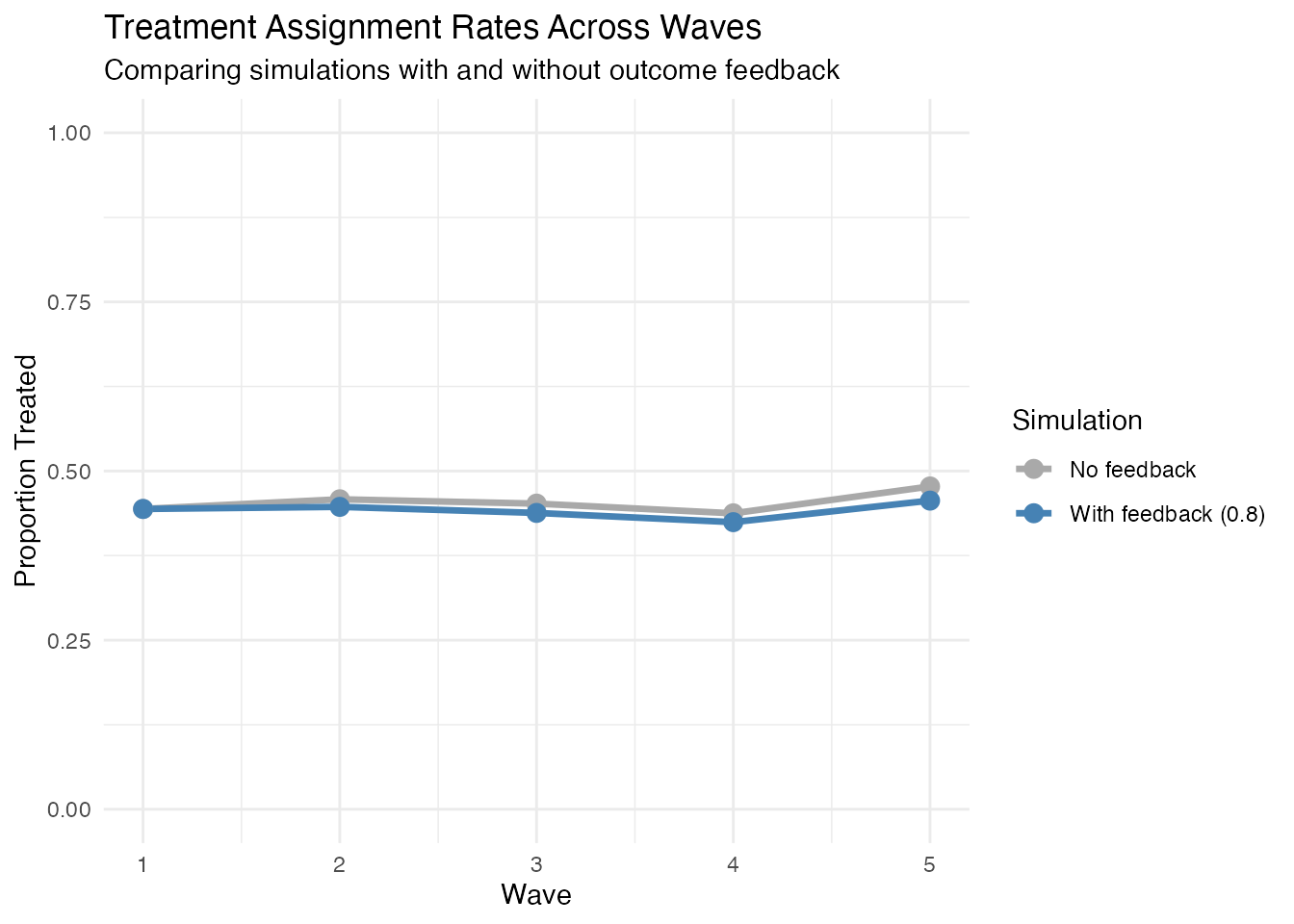
Note: The y_feedback parameter affects how past outcomes
influence future treatment assignment. The specific pattern depends on
the interaction between outcome values, baseline covariates, and the
simulation parameters. In practice, y_feedback creates time-varying
confounding by making treatment assignment depend on past outcomes.
3.4 Positivity diagnostics
Estimators grounded in the g-formula, IPW, or TMLE require sufficient overlap (positivity) of treatment probabilities across strata of measured covariates. Below we inspect estimated propensity scores at the final observed wave in the heterogeneous-effects example.
# wave-3 propensity model: A1 ~ B2
# Filter to complete cases for this analysis
het_complete <- het_dat %>%
  filter(!is.na(t3_A1) & !is.na(B2))

ps_mod <- glm(t3_A1 ~ B2, family = binomial, data = het_complete)
het_complete$ps3 <- predict(ps_mod, type = "response")

ggplot(het_complete, aes(ps3, fill = factor(t3_A1))) +
  geom_histogram(position = "identity", alpha = 0.4, bins = 30) +
  labs(
    x    = "estimated propensity score",
    fill = "A1 at wave 3"
  ) +
  theme_minimal()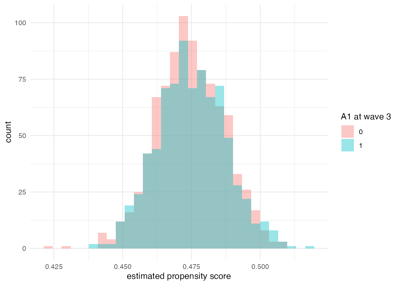
4. Censoring & missingness
Attrition can depend on exposure, a latent frailty shared within individuals, or both. For brevity, see the dedicated Censoring vignette.
5. Power analysis template
Combined heterogeneity and feedback can inflate sample-size requirements. Use batched simulations to trace operating characteristics; skeleton:
power_grid <- tibble::tibble(N = seq(500, 5000, by = 500))

power_grid$power <- vapply(power_grid$N, function(n) {
  mean(replicate(300, {
    dat <- margot_simulate(n = n, waves = 4,
                           y_feedback = 0.7,
                           exposures = list(A1 = list(type = "binary",
                                                      het = list(modifier = "B1", coef = 0.5))),
                           exposure_outcome = 0.3, wide = TRUE))
    t.test(t5_Y ~ t3_A1, data = dat)$p.value < 0.05
  }))
}, numeric(1))

ggplot(power_grid, aes(N, power)) +
  geom_line() +
  geom_hline(yintercept = 0.8, linetype = "dashed") +
  scale_y_continuous(labels = scales::percent_format()) +
  labs(y = "Power", x = "Sample size")