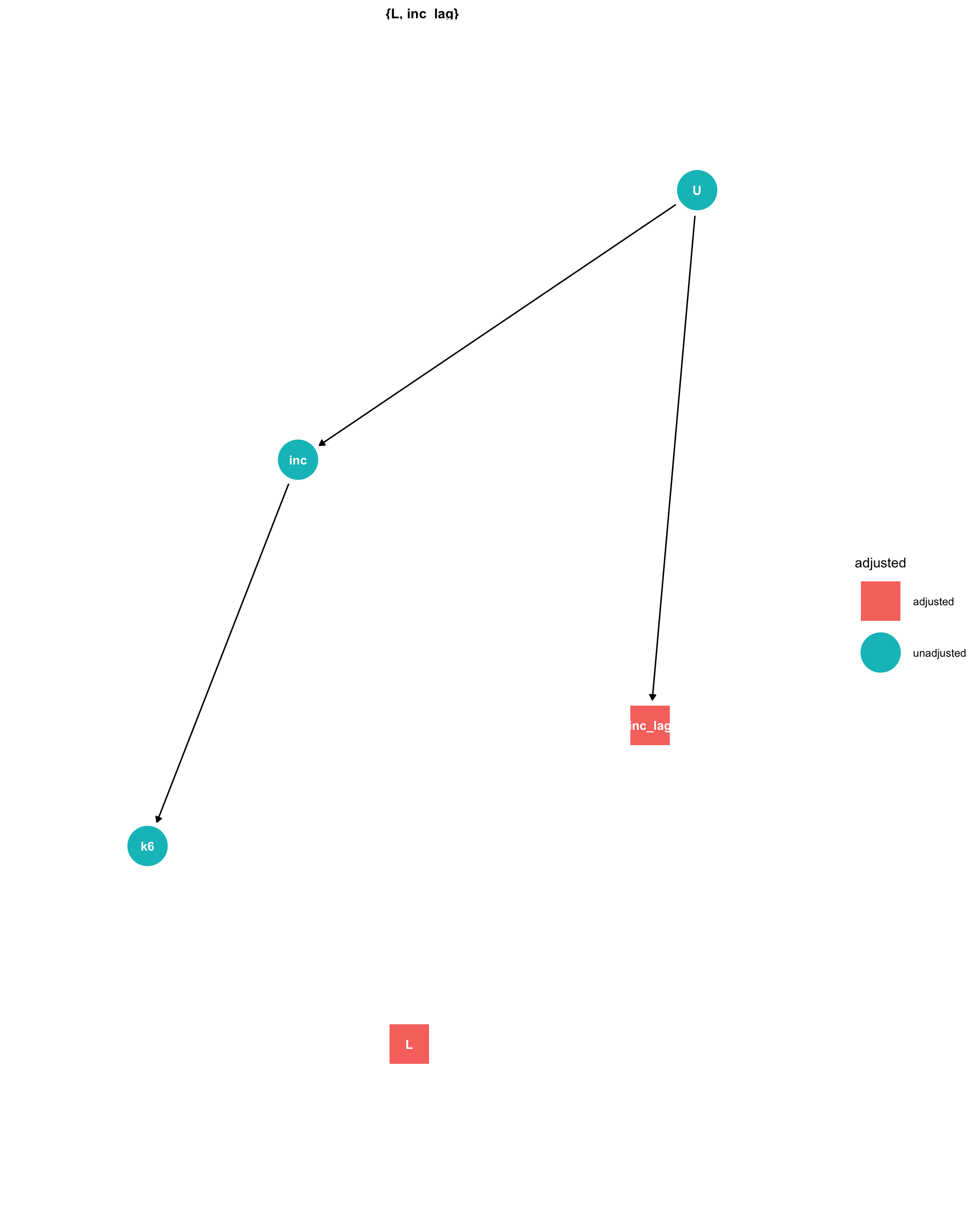
Dag
We adjust for the effects of unmeasured confounders (U) by conditioning on the lag of the exposure, the lag of the outcome, and the lag2 of measured confounders (L):
Show code
# Create Dags
library(ggdag)
dg <- ggdag::dagify(
  k6  ~ inc  + inc_lag +  L ,
  inc_lag ~ L + U,
  inc ~ L + U,
  exposure = "inc",
  outcome = "k6",
  latent = "U"
)

#Check backdoor paths
#p1 <-ggdag(dg) + theme_dag_blank() + labs(title = "confounding control")
#p1
ggdag::ggdag_adjustment_set(dg) + theme_dag_blank()
Descriptive graphs
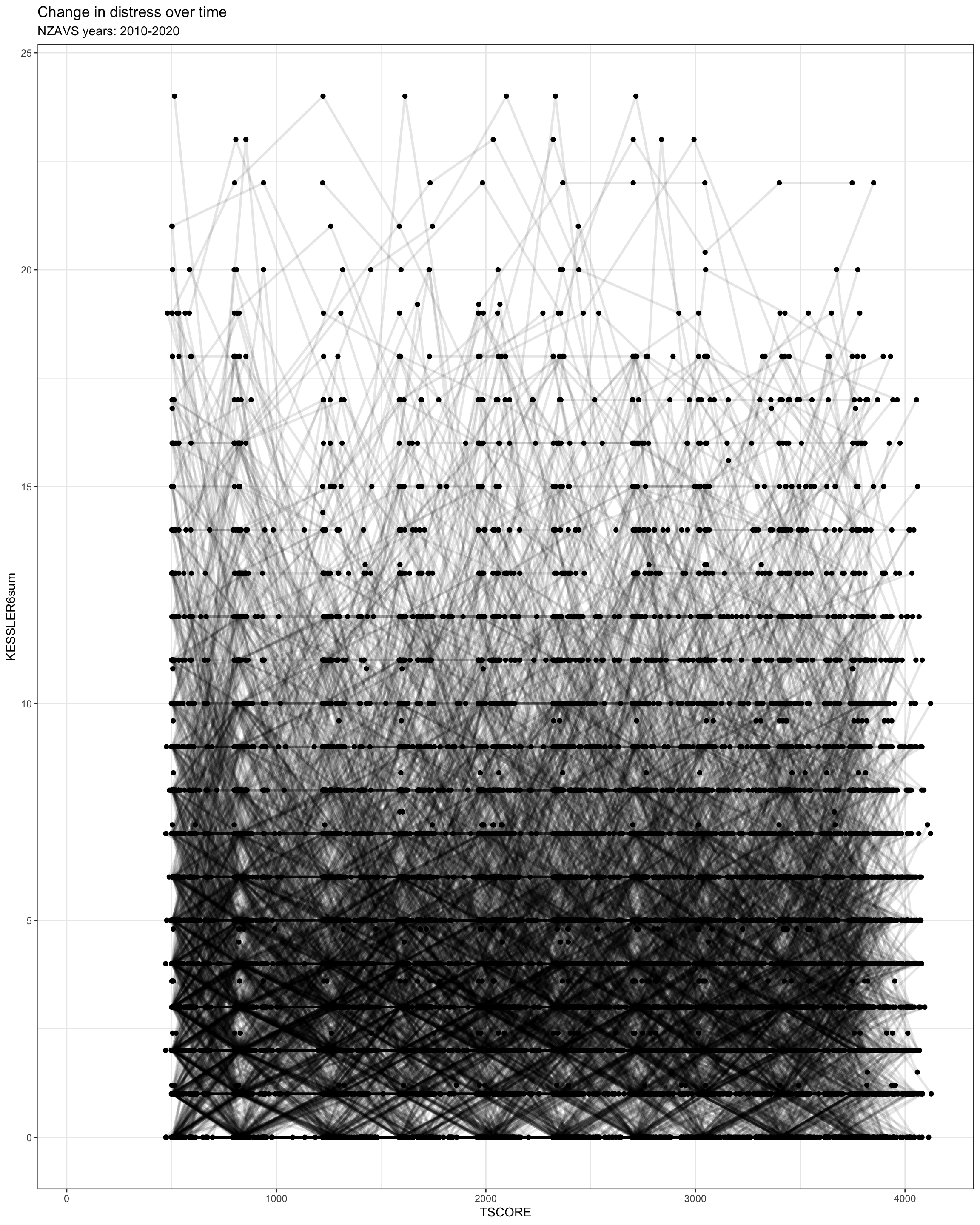
Here we plot change in K6 by id over 10 waves. Hard to see what is happening.
Show code
df %>%
  dplyr::filter(YearMeasured==1) %>%
  dplyr::group_by(Id) %>% filter(n() > 9) %>%
  ungroup()%>%
  ggplot(aes(x = TSCORE,
             y = KESSLER6sum)) +
  geom_point() +
  geom_line(aes(group = Id),
            size = 1,
            alpha = .1) +
 # geom_smooth(method = "lm") +
  theme_bw() +
  #facet_grid(.~ Employed) +
  labs(title = "Change in distress over time",
       subtitle = "NZAVS years: 2010-2020")
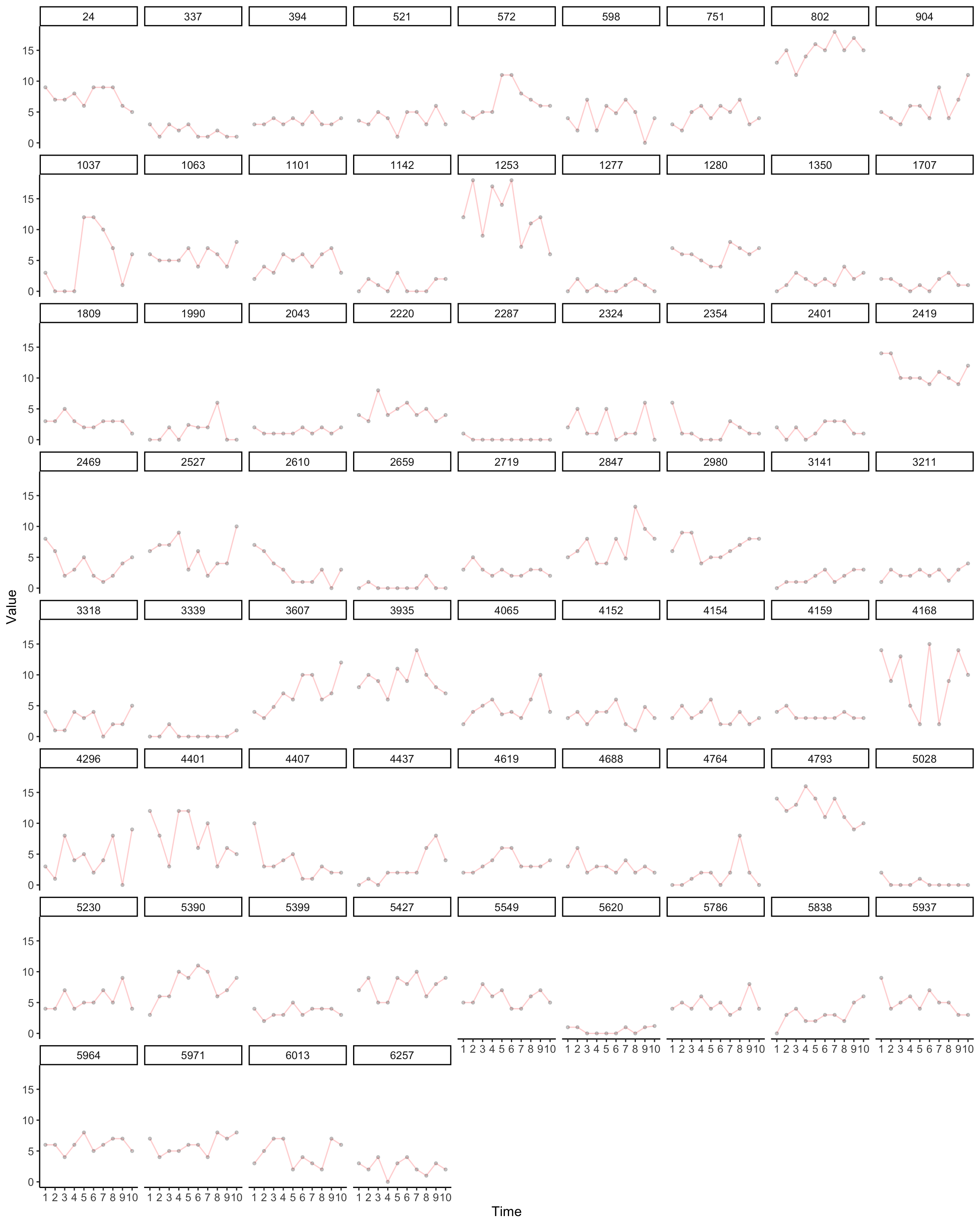
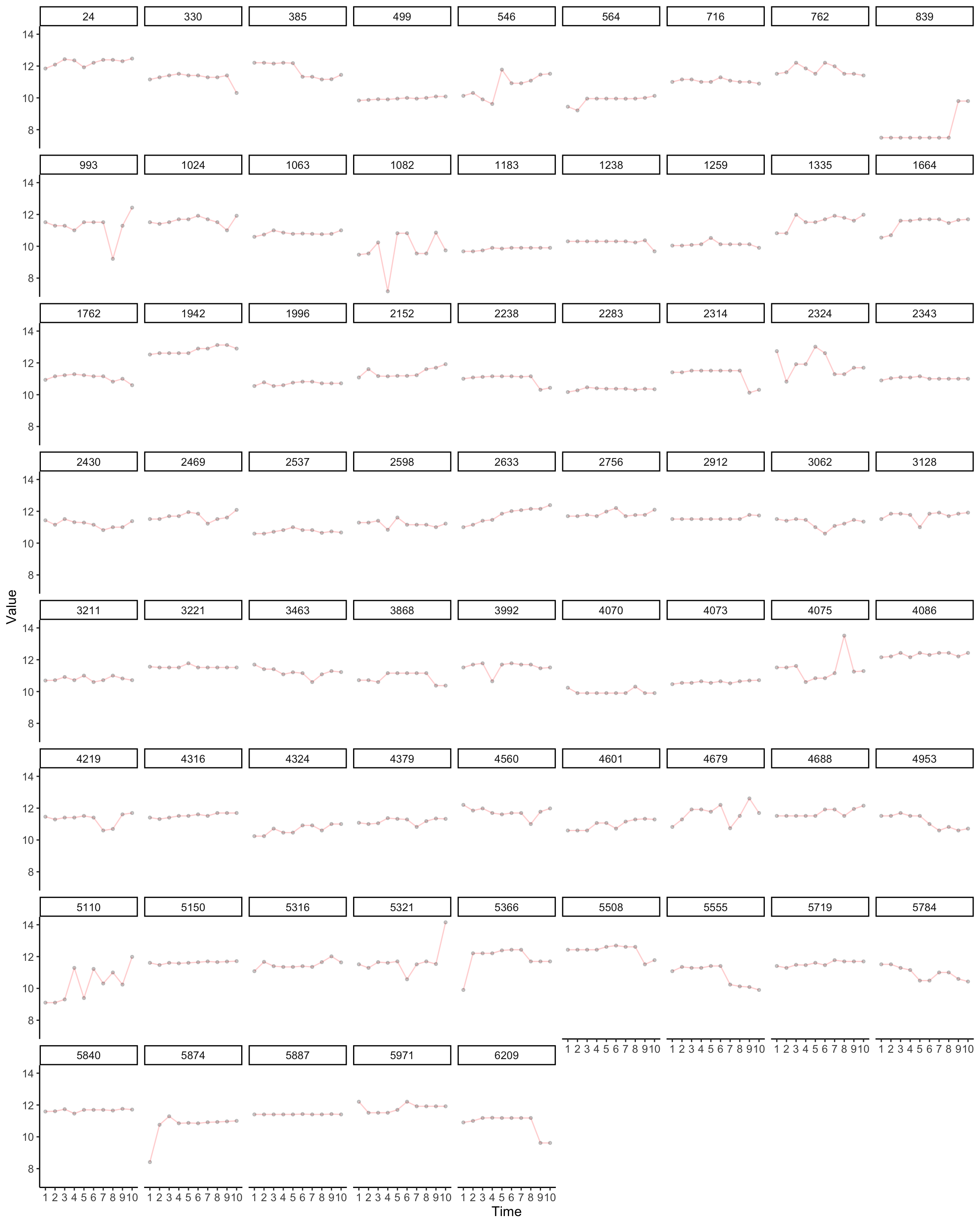
Here we plot distress trajectories witin a subset of individuals. This approach helps us to see the qualities of the data.
Show code
library(lcsm)
widelong <-  df %>%
  dplyr::filter(YearMeasured==1) %>%
  dplyr::filter(Wave!=2009) %>% # k6 not measured in wave 1
  dplyr::group_by(Id) %>% filter(n() > 9) %>%
  dplyr::select(Id, KESSLER6sum, Wave) #


wide <- spread(widelong, Wave, KESSLER6sum)

wide2 <- wide[complete.cases(wide),]


x_var_list <- names(wide2[, 2:11])


wide2 <- as.data.frame(wide2)
plot_trajectories(
  data = wide2,
  id_var = "Id",
  var_list = x_var_list,
  line_colour = "red",
  xlab = "Time",
  ylab = "Value",
  connect_missing = F,
  scale_x_num = T,
  scale_x_num_start = 1,
  random_sample_frac = 0.05,
  seed = 1234
  #title_n = T
)  +
  facet_wrap( ~ Id)
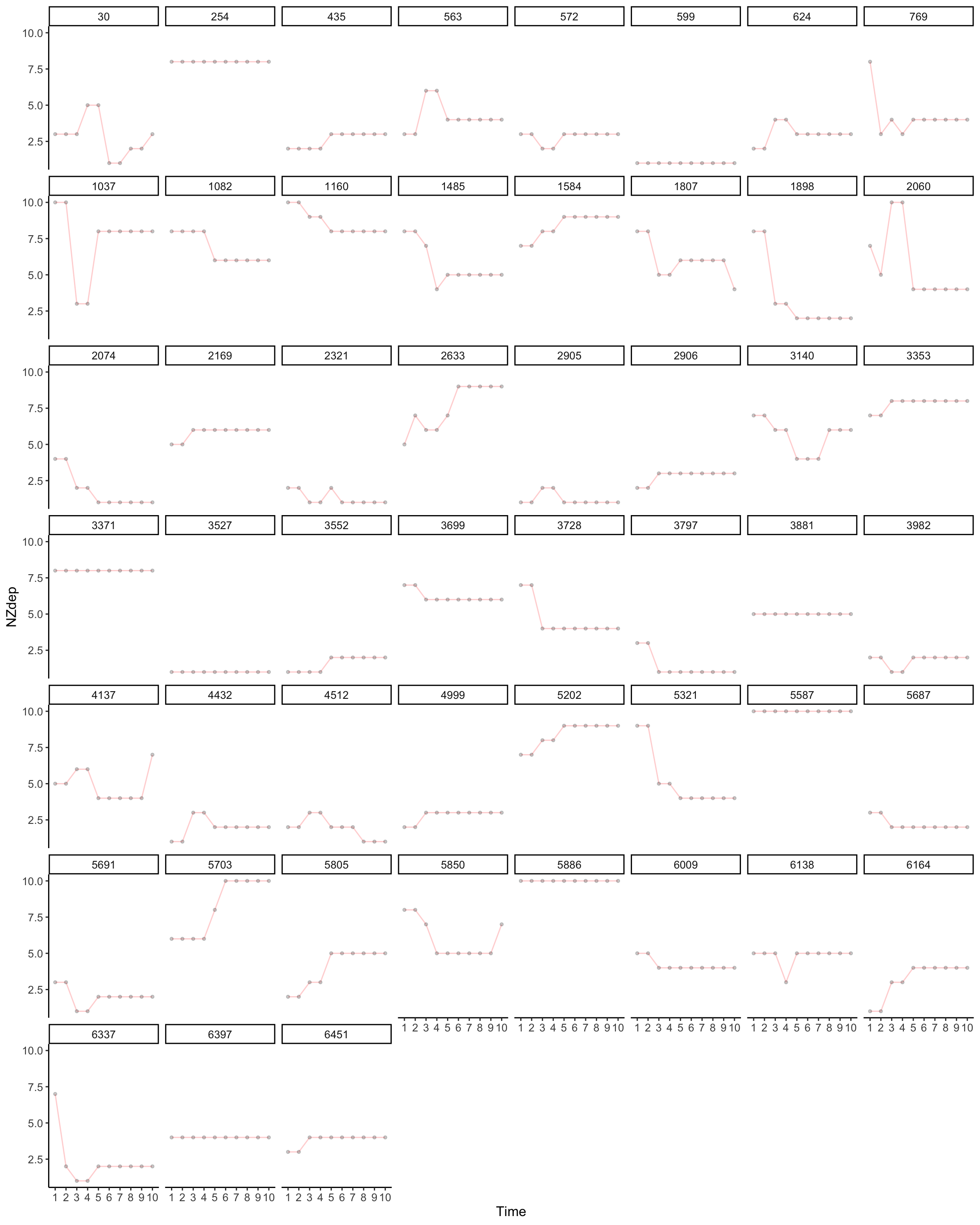
Next we can look at variation in income. Is this variable reliable?
Show code
widelong <-  df %>%
  dplyr::filter(YearMeasured==1) %>%
  dplyr::filter(Wave!=2009) %>% # 1
  dplyr::group_by(Id) %>% filter(n() > 9) %>%
  dplyr::ungroup() %>%
  dplyr::mutate(Household.INC_log = log(Household.INC+1)) %>%
  dplyr::select(Id, Household.INC_log, Wave) #

wide <- spread(widelong, Wave, Household.INC_log)

wide2 <- wide[complete.cases(wide),]


x_var_list <- names(wide2[, 2:11])
wide2 <- as.data.frame(wide2) # needs df

# graph
plot_trajectories(
  data = wide2,
  id_var = "Id",
  var_list = x_var_list,
  line_colour = "red",
  xlab = "Time",
  ylab = "Value",
  connect_missing = F,
  scale_x_num = T,
  scale_x_num_start = 1,
  random_sample_frac = 0.05,
  seed = 1234
  #title_n = T
)  +
  facet_wrap( ~ Id)
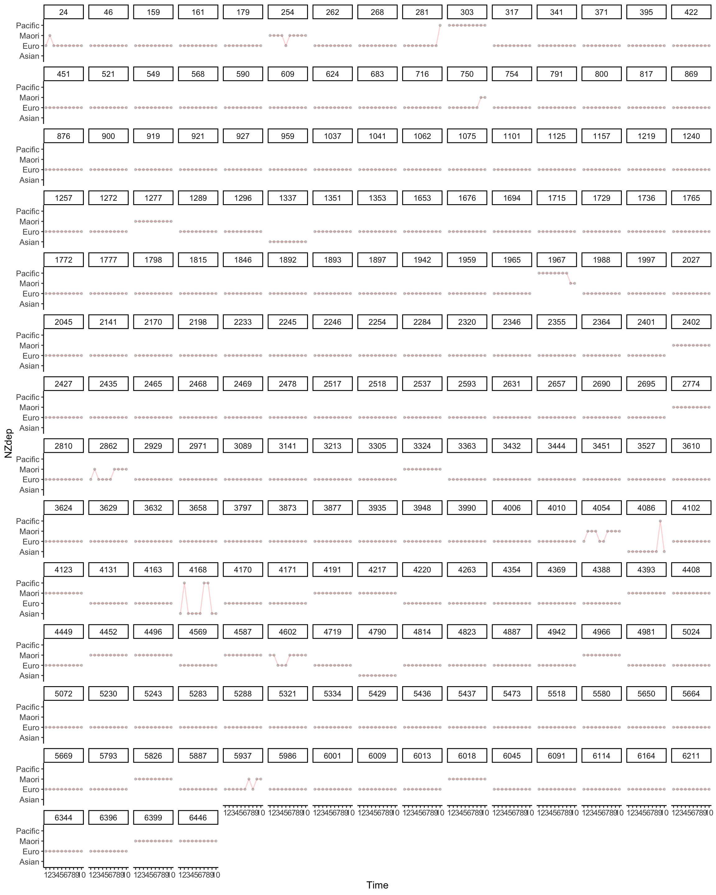
Consider NZdep. Is this variable reliable? Lots of movement. Household income is better
Show code
widelong <-  df %>%
  dplyr::filter(YearMeasured==1) %>%
  dplyr::filter(Wave!=2009) %>% # 1
  dplyr::group_by(Id) %>% filter(n() > 9) %>%
  dplyr::ungroup() %>%
  dplyr::select(Id, NZdep, Wave) #

wide <- spread(widelong, Wave, NZdep)


wide2 <- wide[complete.cases(wide),]


x_var_list <- names(wide2[, 2:11])


wide2 <- as.data.frame(wide2)
plot_trajectories(
  data = wide2,
  id_var = "Id",
  var_list = x_var_list,
  line_colour = "red",
  xlab = "Time",
  ylab = "NZdep",
  connect_missing = F,
  scale_x_num = T,
  scale_x_num_start = 1,
  random_sample_frac = 0.05,
  seed = 1234
  #title_n = T
)  +
  facet_wrap( ~ Id)
Prepare data
What might affect both income and happiness?
L = ethnicity, male, partner (current, lag), cohort, NZdep?, urban, employed edu (too much missingness).
Show code
dg <- df %>%
  dplyr::filter(YearMeasured == 1)  %>%
  dplyr::filter(Wave != 2009) %>% # no k6 measure
  dplyr::filter(!is.na(Household.INC), !is.na(KESSLER6sum)) %>%
  dplyr::group_by(Id) %>% filter(n() > 2) %>% ungroup() %>%
  dplyr::filter(Household.INC > 10000) %>%  # retired people, people in care  %>%
  dplyr::mutate(inc_quant = ntile(Household.INC, 4)-1) %>% # income categories
  # dplyr::mutate(k6_cats = cut(
  #   KESSLER6sum,
  #   breaks = c(-Inf, 5, 13, Inf),
  #   # create Kessler 6 diagnostic categories
  #   labels = c("Low Distress", "Moderate Distress", "Serious Distress"),
  #   right = TRUE
  # )) %>%
  dplyr::mutate(k6 =  as.numeric(KESSLER6sum) ) %>%
  dplyr::select(Id,
                inc_quant,
                k6,
                Wave,
                GenCohort,
                Euro,
                Religious,
                Male,
                Urban,
                Employed,
                Household.INC,
                Partner) %>%
  dplyr::mutate(across(
    c(inc_quant,
      k6,
      Employed,
      Religious,
      Urban,
      Partner),
    list(lag = lag)
  )) %>%
  drop_na() %>%
  dplyr::arrange(Id, Wave) %>%
  dplyr::group_by(Id) %>%
  mutate(time = (as.numeric(Wave) - min(as.numeric(Wave)))) %>% # zero time is start for each person
  dplyr::ungroup(Id)


#dt<- dt %>%
 # mutate_all(~as.numeric(.))

# number of participants
length(unique(dg$Id))
[1] 21764Inspect our cutpoints
Show code
# A tibble: 4 × 3
inc_quant min_inc max_inc
<dbl> <dbl> <dbl>
1 0 10036 53300
2 1 53480 90000
3 2 90000 140000
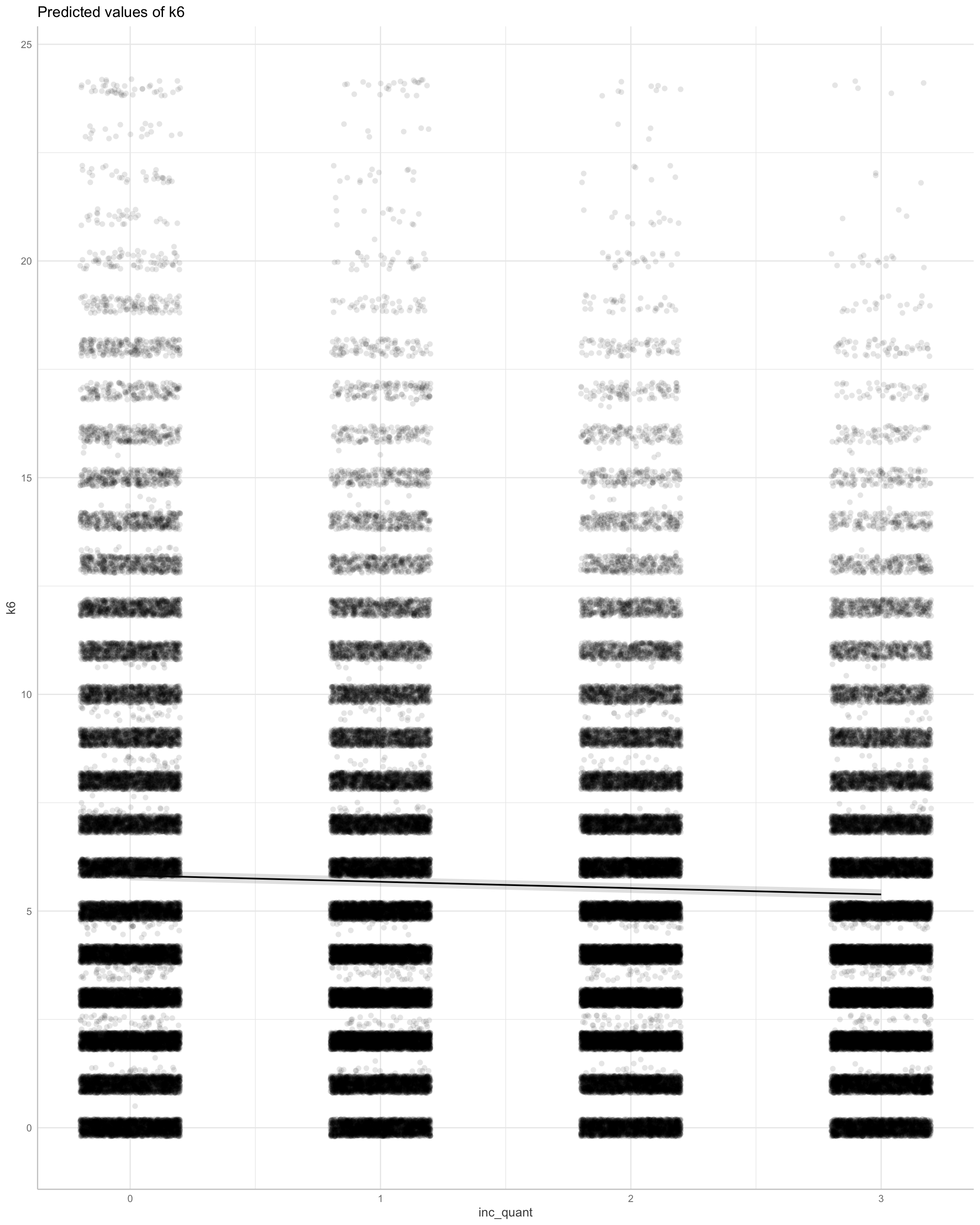
4 3 140000 3500000Marginal structural model
First we create weights
Show code
dg_w <- ipw::ipwtm(
exposure = inc_quant,
family = "ordinal",
link = "probit",
type = "first",
corstr = "ar1",
id = "Id",
timevar = "time",
numerator = ~
inc_quant_lag + # lag treatment + time invariant confounders
GenCohort +
Male +
Euro, #+
denominator = ~ # lag treatment + lag outcome + confounders +
inc_quant_lag +
k6_lag +
GenCohort +
Male +
Urban +
Euro +
Partner +
Partner_lag +
Employed +
Employed_lag,
data = as.data.frame(dg)
)
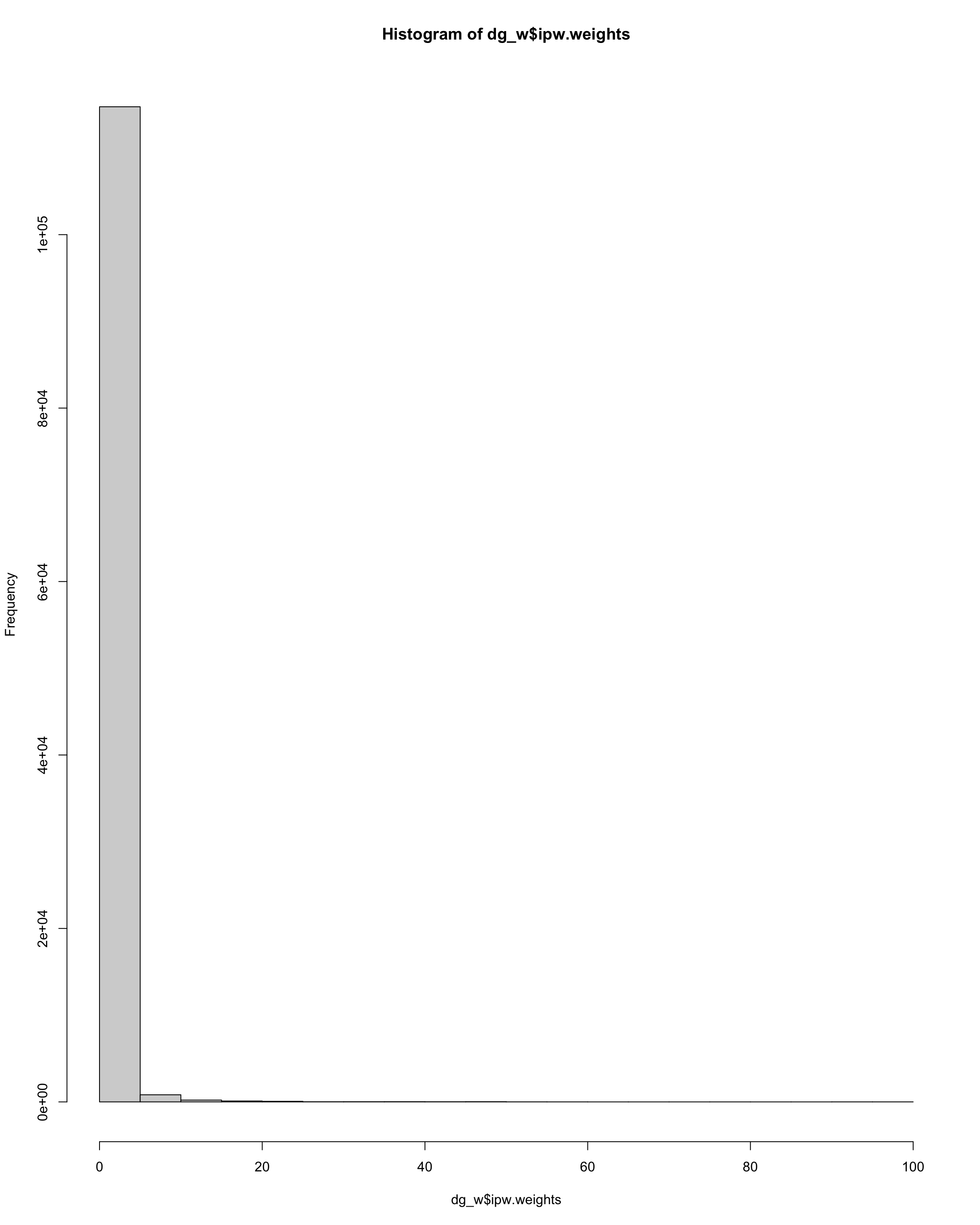
hist(dg_w$ipw.weights)
Show code
sum(dg_w$ipw.weights > 10)
[1] 494Show code
## GEE
m0 <- geeglm(
  k6  ~
     inc_quant +
     inc_quant_lag,
  data = dg_w_use,
  id = Id,
  family = "gaussian",
  weights = ipw,
  waves = time,
  corstr = "ar1"
)

parameters::model_parameters(m0) %>%
  print_html()
| Model Summary | |||||
|---|---|---|---|---|---|
| Parameter | Coefficient | SE | 95% CI | Chi2(1) | p |
| (Intercept) | 5.34 | 0.05 | (5.23, 5.44) | 9802.81 | < .001 |
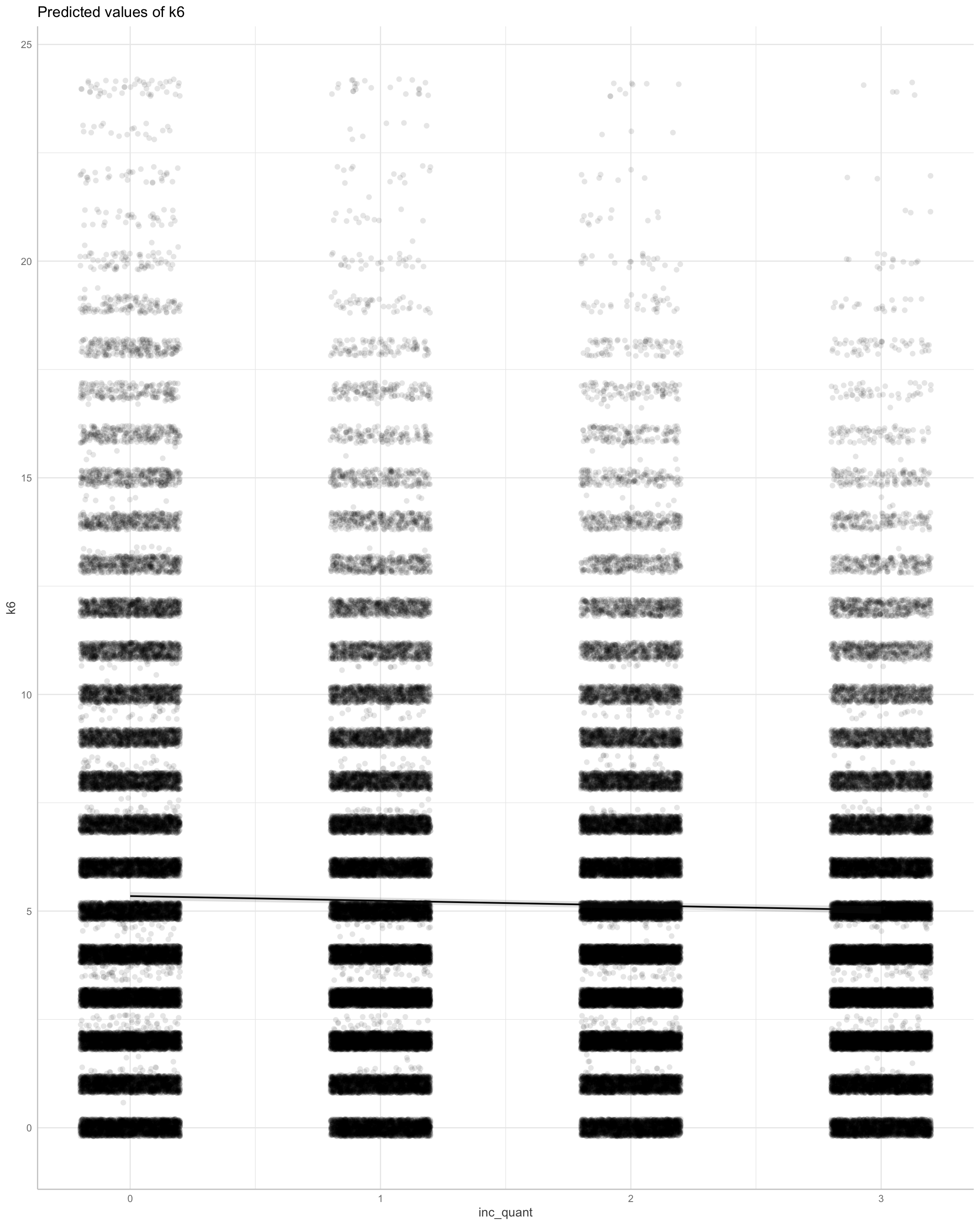
| inc quant | -0.11 | 0.02 | (-0.14, -0.07) | 31.58 | < .001 |
| inc quant lag | 5.84e-03 | 0.02 | (-0.02, 0.04) | 0.14 | 0.704 |
Show code

GEE no weights
Show code
# cannot plot without weights. so we add very small amount of noise
dg_w_use$nullwts  <- rnorm(nrow(dg_w_use), 1,.001)


m0b <- geeglm(
  k6  ~
     k6_lag +
     inc_quant +
     inc_quant_lag  +
     GenCohort +
     Male +
     Urban +
     Euro +
     Partner +
     Partner_lag +
     Employed +
     Employed_lag,
  data = dg_w_use,
  id = Id,
  family = "gaussian",
  weights = nullwts,
  waves = time,
  corstr = "ar1"
)

parameters::model_parameters(m0b) %>%
  print_html()
| Model Summary | |||||
|---|---|---|---|---|---|
| Parameter | Coefficient | SE | 95% CI | Chi2(1) | p |
| (Intercept) | 5.93 | 0.12 | (5.68, 6.17) | 2314.14 | < .001 |
| k6 lag | -0.25 | 3.35e-03 | (-0.26, -0.24) | 5627.28 | < .001 |
| inc quant | -0.13 | 0.01 | (-0.16, -0.10) | 76.67 | < .001 |
| inc quant lag | -0.06 | 0.01 | (-0.08, -0.04) | 31.12 | < .001 |
| GenCohortGen Boomers * born >= 1946 & b < 1965 | 1.07 | 0.11 | (0.86, 1.28) | 99.65 | < .001 |
| GenCohortGenX * born >=1961 & b < 1981 | 2.26 | 0.11 | (2.04, 2.48) | 408.58 | < .001 |
| GenCohortGenY * born >=1981 & b < 1996 | 3.89 | 0.12 | (3.65, 4.13) | 1004.69 | < .001 |
| GenCohortGenZ * born >= 1996 | 5.01 | 0.35 | (4.32, 5.70) | 202.63 | < .001 |
| Male (Male) | -0.09 | 0.05 | (-0.20, 0.01) | 3.01 | 0.083 |
| Urban (Urban) | -0.01 | 0.03 | (-0.08, 0.05) | 0.11 | 0.736 |
| Euro | -0.33 | 0.06 | (-0.44, -0.22) | 35.66 | < .001 |
| Partner | -0.55 | 0.05 | (-0.65, -0.46) | 137.55 | < .001 |
| Partner lag | -0.17 | 0.03 | (-0.23, -0.10) | 28.08 | < .001 |
| Employed (1) | -0.30 | 0.03 | (-0.37, -0.23) | 75.25 | < .001 |
| Employed lag (1) | -0.03 | 0.03 | (-0.08, 0.03) | 0.96 | 0.326 |
Show code
Multilevel model
Show code
m0c<- lmer(
  k6  ~
     k6_lag +
     inc_quant +
     inc_quant_lag  +
     GenCohort +
     Male +
     Urban +
     Euro +
     Partner +
     Partner_lag +
     Employed +
     Employed_lag +
    (1|Id),
  data = dg_w_use
)

parameters::model_parameters(m0c) %>%
  print_html()
| Model Summary | |||||
|---|---|---|---|---|---|
| Parameter | Coefficient | SE | 95% CI | t(115548) | p |
| Fixed Effects | |||||
| (Intercept) | 4.32 | 0.10 | (4.13, 4.52) | 43.08 | < .001 |
| k6 lag | 0.06 | 2.43e-03 | (0.06, 0.07) | 26.76 | < .001 |
| inc quant | -0.15 | 0.01 | (-0.17, -0.12) | -11.96 | < .001 |
| inc quant lag | -1.31e-03 | 9.96e-03 | (-0.02, 0.02) | -0.13 | 0.895 |
| GenCohortGen Boomers * born >= 1946 & b < 1965 | 0.92 | 0.09 | (0.74, 1.09) | 10.07 | < .001 |
| GenCohortGenX * born >=1961 & b < 1981 | 1.86 | 0.09 | (1.67, 2.04) | 19.77 | < .001 |
| GenCohortGenY * born >=1981 & b < 1996 | 3.21 | 0.10 | (3.01, 3.41) | 31.61 | < .001 |
| GenCohortGenZ * born >= 1996 | 4.19 | 0.27 | (3.67, 4.71) | 15.71 | < .001 |
| Male (Male) | -0.08 | 0.04 | (-0.16, 7.19e-03) | -1.79 | 0.073 |
| Urban (Urban) | 0.01 | 0.02 | (-0.04, 0.06) | 0.45 | 0.654 |
| Euro | -0.31 | 0.04 | (-0.40, -0.22) | -7.00 | < .001 |
| Partner | -0.61 | 0.03 | (-0.68, -0.55) | -18.34 | < .001 |
| Partner lag | 0.10 | 0.03 | (0.05, 0.15) | 3.90 | < .001 |
| Employed (1) | -0.30 | 0.03 | (-0.36, -0.25) | -11.16 | < .001 |
| Employed lag (1) | 5.58e-03 | 0.02 | (-0.04, 0.05) | 0.24 | 0.813 |
| Random Effects | |||||
| SD (Intercept: Id) | 2.83 | ||||
| SD (Residual) | 2.23 | ||||
Show code
Try another approach (older material)
Show code
# prepare data
# note, still need to do IPW and multiply impute missing data

dl <- df %>%
  dplyr::filter(YearMeasured == 1)  %>%
  dplyr::filter(Wave != 2009) %>% # no k6 measure
  dplyr::filter(!is.na(KESSLER6sum), !is.na(Household.INC),!is.na(EthnicCats),!is.na(Male),!is.na(Urban), !is.na(Employed)) %>%
  dplyr::filter(Household.INC > 10000 ) %>%  # retired people, people in care
  dplyr::select(
    Id,
    Household.INC,
    KESSLER6sum,
    NZdep,
    Wave,
    TSCORE,
    Age,
    Religious,
    Religion.Church,
    Male,
    Edu,
    EthnicCats,
    Urban,
    Wave,
    Employed,
    Partner
  ) %>%
  dplyr::mutate(
    k6 = as.numeric(KESSLER6sum),
    age = (Age),
    inc_l = log(Household.INC + 1),
    emp = as.numeric(Employed),
  #  pray_l = log(Religion.Prayer + 1),
  #  script_l = log(Religion.Scripture + 1),
    church_l = log(Religion.Church + 1),
    edu = as.numeric(Edu),
    religious = as.numeric(Religious),
    partner = as.numeric(Partner),
    male = as.factor(Male),
    eth = EthnicCats,
    nzdep = as.numeric(NZdep),
    urban = Urban,
   id = Id
  ) %>%
  dplyr::group_by(Id) %>% filter(n() > 2) %>%
  mutate(time0 = as.numeric(Wave))%>%
  dplyr::mutate(across(
    c(
      age,
      male,
      eth,
      emp,
      urban,
      k6,
      inc_l,
      edu,
      church_l,
      nzdep,
      partner,
      religious
    ),
    list(lag = lag) )) %>%
  #  dplyr::mutate(across(c(age_lag,
  #                       eth_lag,
  #                       urban_lag,
  #                       male_lag,
  #                       urban_lag,
  #                       edu_lag,
  #                       church_l_lag,
  #                       nzdep_lag,
  #                       partner_lag,
  #                       religious_lag,
  #                       emp_lag,
  #                       inc_l_lag,
  #                       k6_lag),
  #                list(lag = lag)
  #                ))%>%
   dplyr::ungroup(Id) %>%
   dplyr::select(id, k6, k6_lag, inc_l_lag, age_lag, eth_lag,urban_lag,
                 church_l_lag, nzdep_lag, church_l, partner, partner_lag, emp_lag, male_lag, inc_l, Id, Wave) %>%
  drop_na() %>%
  dplyr::arrange(Id, Wave) %>%
  dplyr::group_by(Id) %>%
  mutate(time = (as.numeric(Wave) - min(as.numeric(Wave)))) %>% # zero time is start for each person
  dplyr::ungroup(Id)

#dt<- dt %>%
 # mutate_all(~as.numeric(.))

dl <- as.data.frame(dl)
Number of participants
Prepare data for IP Weights
Show code
## Marginal Structural model approach: IPW
# calculate weights: Note -- is this correct?
# example type ?ipwtm
dl_weights_2 <- ipw::ipwtm(
  exposure = inc_l,
  family = "gaussian",
  type = "all",
  corstr = "ar1",
  id = "id",
  timevar = "time",
  numerator = ~  inc_l_lag  +  # lag treatment + time invariant confounders
     age_lag +
     male_lag +
     eth_lag +
     emp_lag +
     nzdep_lag +
     urban_lag,
  denominator = ~ # lag treatment + lag outcome +  confounders
     k6_lag  +
     inc_l_lag  +
     age_lag +
     male_lag +
     eth_lag +
     emp_lag +
     nzdep_lag +
     urban_lag +
     partner_lag, # household income
  data = as.data.frame(dl)
)

sum(dl_weights_2$ipw.weights > 10)
[1] 0Show code
hist(dl_weights_2$ipw.weights)
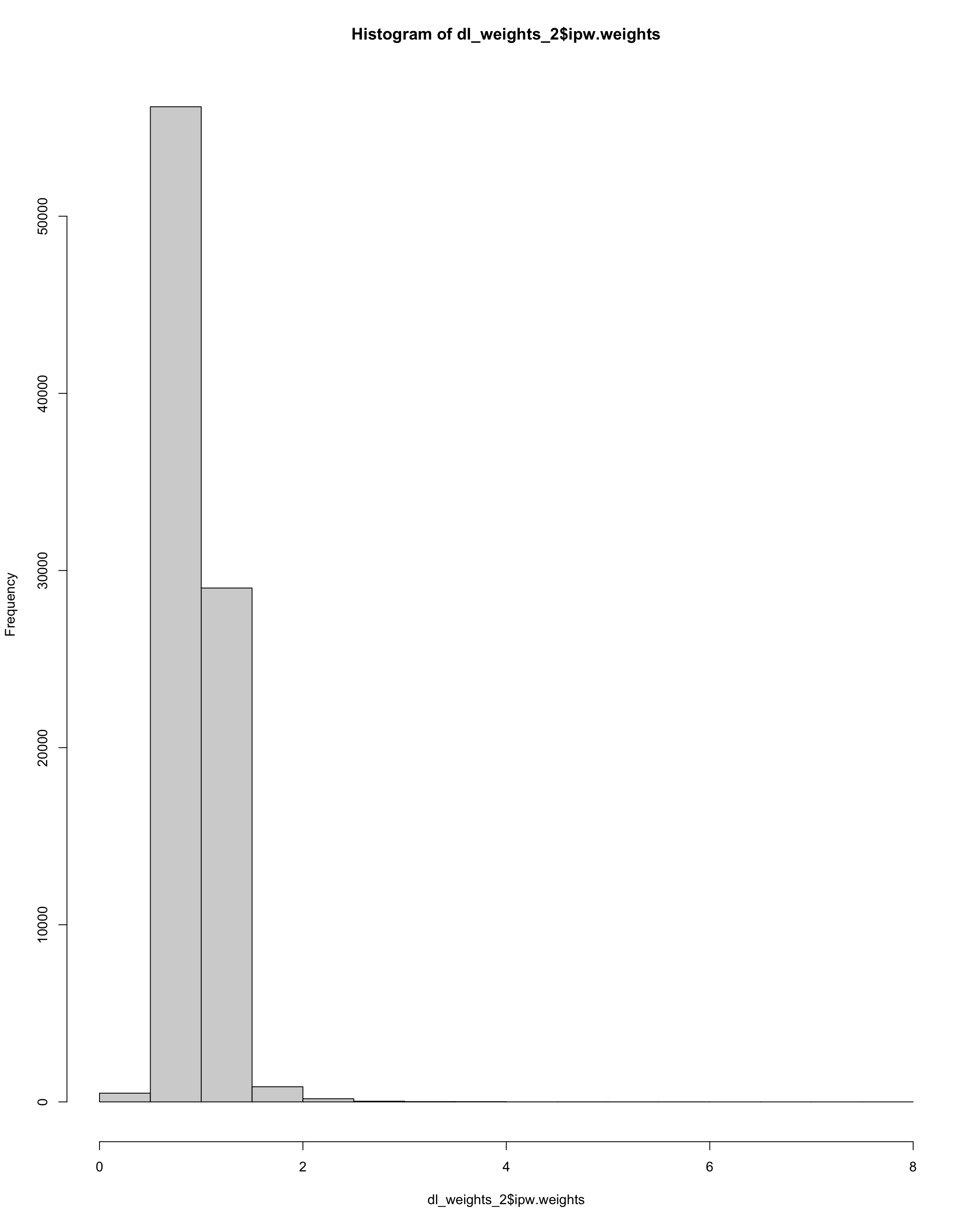
Check weights – this looks pretty extreme
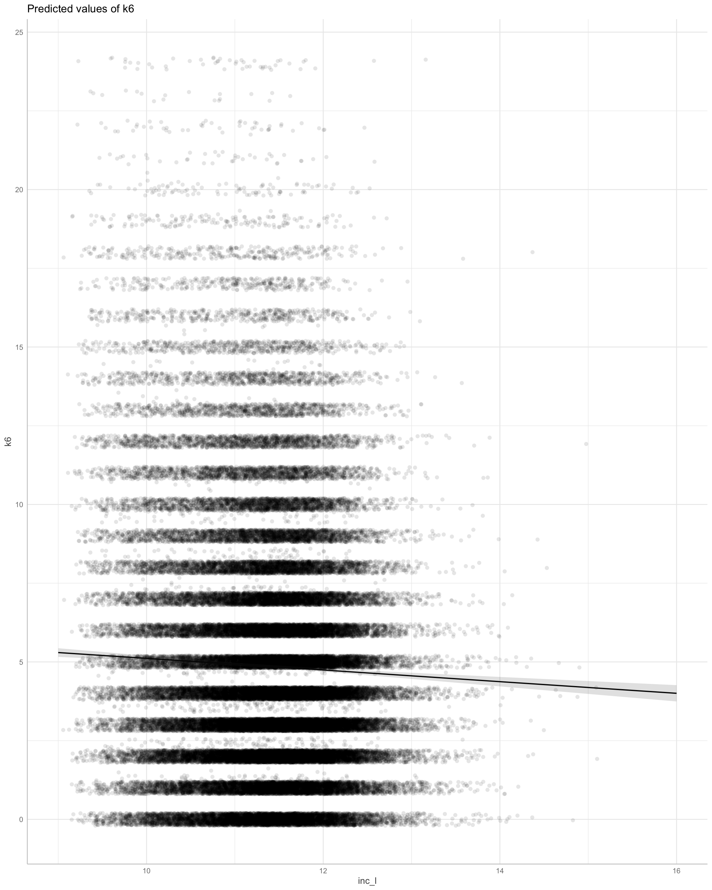
GEE
Note that we incorportate the covarariates into “weights”
Show code
## GEE

m2z <- geeglm(
  k6  ~
    inc_l +
    inc_l_lag,
  data = dl_weights_use_2,
  id = id,
  weights = ipw,
  waves = time,
  corstr = "ar1"
)

parameters::model_parameters(m2z) %>%
  print_html()
| Model Summary | |||||
|---|---|---|---|---|---|
| Parameter | Coefficient | SE | 95% CI | Chi2(1) | p |
| (Intercept) | 8.29 | 0.39 | (7.52, 9.06) | 441.53 | < .001 |
| inc l | -0.13 | 0.03 | (-0.20, -0.07) | 17.79 | < .001 |
| inc l lag | -0.15 | 0.03 | (-0.22, -0.09) | 22.98 | < .001 |
Show code
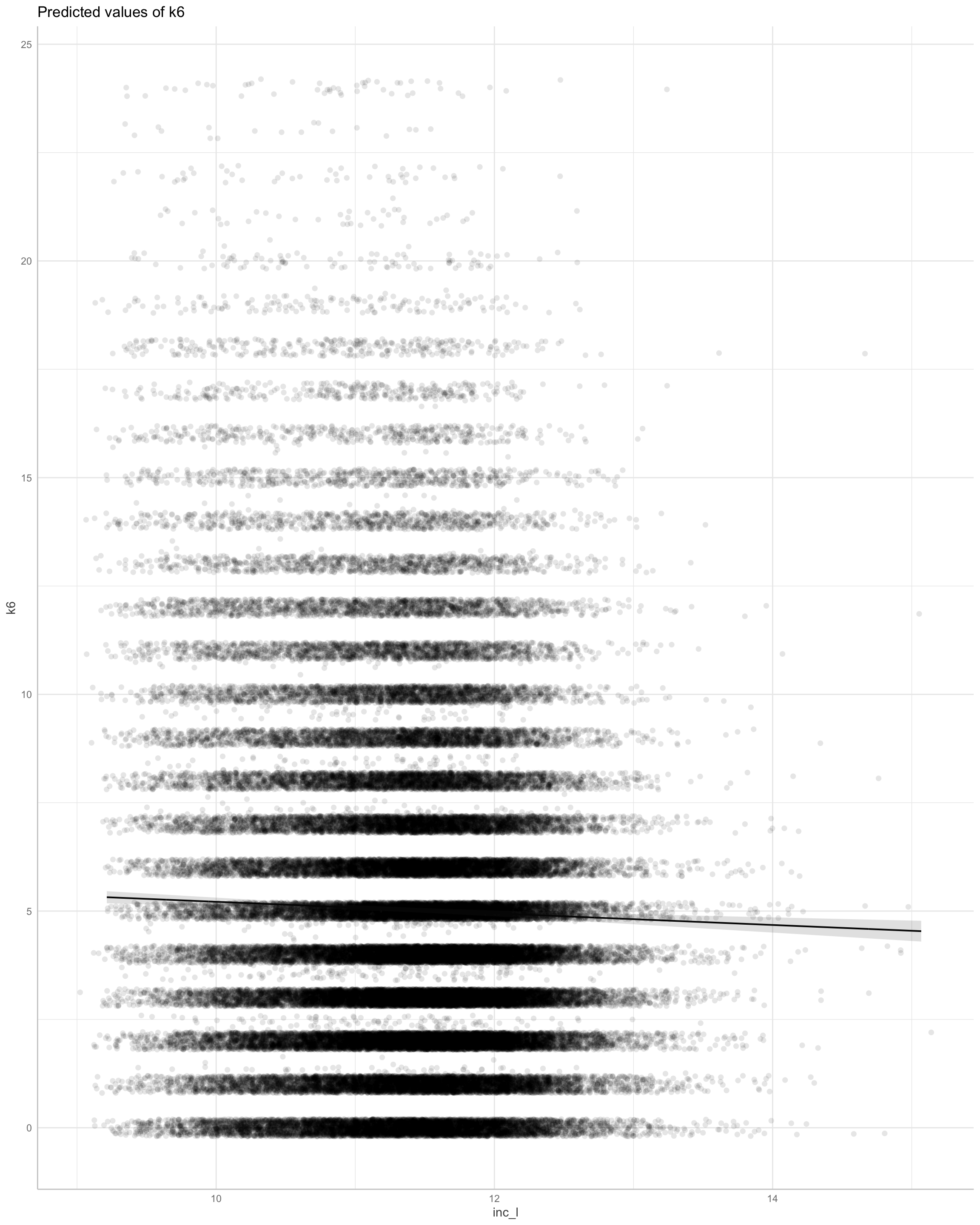
Weights yeilds an attenuated effect. *Highly sensitive to model misspecification**
GEE without weights
Show code
## GEE
str(dt)
function (x, df, ncp, log = FALSE) Show code
# cannot plot without weights. so we add very small amount of noise
dl_weights_use_2$nullwts  <- rnorm(nrow(dl_weights_use_2), 1,.001)


m2z2 <- geeglm(
  k6  ~
     k6_lag +
     inc_l +
     inc_l_lag  +
     age_lag +
     partner_lag +
     male_lag +
     eth_lag +
     emp_lag +
     nzdep_lag +
     urban_lag,
  data = dl_weights_use_2,
  id = id,
  weights = nullwts,
  waves = time,
  corstr = "ar1"
)

parameters::model_parameters(m2z2) %>%
  print_html()
| Model Summary | |||||
|---|---|---|---|---|---|
| Parameter | Coefficient | SE | 95% CI | Chi2(1) | p |
| (Intercept) | 3.89 | 0.16 | (3.57, 4.21) | 576.06 | < .001 |
| k6 lag | 0.78 | 3.28e-03 | (0.77, 0.78) | 55855.33 | < .001 |
| inc l | -0.18 | 0.03 | (-0.24, -0.13) | 42.69 | < .001 |
| inc l lag | 0.02 | 0.03 | (-0.04, 0.07) | 0.31 | 0.575 |
| age lag | -0.02 | 6.55e-04 | (-0.02, -0.02) | 728.91 | < .001 |
| partner lag | 2.91e-03 | 0.02 | (-0.04, 0.04) | 0.02 | 0.886 |
| male lag (Male) | 4.10e-03 | 0.02 | (-0.03, 0.03) | 0.07 | 0.785 |
| eth lag (Maori) | -0.01 | 0.02 | (-0.06, 0.04) | 0.25 | 0.617 |
| eth lag (Pacific) | 0.02 | 0.06 | (-0.10, 0.14) | 0.12 | 0.729 |
| eth lag (Asian) | 0.03 | 0.04 | (-0.05, 0.12) | 0.55 | 0.456 |
| emp lag | -0.06 | 0.02 | (-0.10, -0.02) | 7.41 | 0.006 |
| nzdep lag | 0.01 | 2.94e-03 | (8.97e-03, 0.02) | 25.07 | < .001 |
| urban lag (Urban) | 0.08 | 0.02 | (0.04, 0.11) | 21.45 | < .001 |
Show code
Does money make people happy?
Lingering Questions:
- What is the target-trial that we are trying to emulate here? (cf Hernans…)
- exposure/outcome confounding?
- do we want to define a clear treatment (ordinal categories for income?), so that we can emulate a target trial and obtain better IPW?
Older material:
Show code
# comparative analysis
# prepare data
# note, still need to do IPW and multiply impute missing data
dt <- df %>%
  dplyr::filter(YearMeasured == 1)  %>%
 dplyr::filter(Wave != 2009) %>% # no k6 measure
  dplyr::filter(!is.na(KESSLER6sum), !is.na(Household.INC),!is.na(EthnicCats),!is.na(Male),!is.na(Urban), !is.na(Employed)) %>%
  dplyr::filter(Household.INC > 10000) %>%
  dplyr::select(
    Id,
    Household.INC,
    KESSLER6sum,
    NZdep,
    Wave,
    TSCORE,
    Age,
    Religious,
    Religion.Prayer,
    Religion.Scripture,
    Religion.Church,
    Male,
    Edu,
    EthnicCats,
    Urban,
    Wave,
    Employed,
    Partner
  ) %>%
  dplyr::mutate(
    k6 = as.numeric(KESSLER6sum),
    age = (Age),
    inc_l = log(Household.INC + 1),
    emp = as.numeric(Employed),
  #  pray_l = log(Religion.Prayer + 1),
  #  script_l = log(Religion.Scripture + 1),
    church_l = log(Religion.Church + 1),
    edu = as.numeric(Edu),
    religious = as.numeric(Religious),
    partner = as.numeric(Partner),
    male = as.factor(Male),
    eth = EthnicCats,
    nzdep = as.numeric(NZdep),
    urban = Urban,
   id = Id
  ) %>%
  dplyr::group_by(Id) %>% filter(n() > 2) %>%
  dplyr::mutate(across(
    c(
      age,
      male,
      eth,
      emp,
      urban,
      k6,
      inc_l,
      edu,
      church_l,
      nzdep,
      partner,
      religious
    ),
    list(lag = lag)
  )) %>%
   dplyr::mutate(across(c(age_lag,
                        eth_lag,
                        urban_lag,
                        male_lag,
                        urban_lag,
                        edu_lag,
                        church_l_lag,
                        nzdep_lag,
                        partner_lag,
                        religious_lag,
                        emp_lag,
                        inc_l_lag,
                        k6_lag),
                 list(lag = lag)
                 ))%>%
  dplyr::ungroup(Id) %>%
  dplyr::select(id, k6, k6_lag, inc_l_lag, age_lag_lag, eth_lag_lag,urban_lag_lag,edu_lag_lag,
                church_l_lag_lag,nzdep_lag_lag,partner_lag_lag,emp_lag_lag,male_lag_lag, inc_l, age_lag, emp_lag, partner_lag,male_lag, edu_lag, eth_lag, church_l_lag, urban_lag, religious_lag, nzdep_lag, inc_l_lag_lag, Id, Wave) %>%
  drop_na() %>%
  dplyr::arrange(Id, Wave) %>%
  dplyr::group_by(Id) %>%
  mutate(time = (as.numeric(Wave) - min(as.numeric(Wave)))) %>% # zero time is start for each person
  dplyr::ungroup(Id)


#dt<- dt %>%
 # mutate_all(~as.numeric(.))


dt<-as.data.frame(dt)
Number of participants
Prepare data for within/between models
Some worry about “heterogeneity bias.” Can separate within and between participant features of change? It seems that we should do so, for example, to avoid Simpson’s Paradoxes.
See: https://easystats.github.io/datawizard/articles/demean.html
Prepare data for IP Weights
Show code
## Marginal Structural model approach: IPW
# calculate weights: Note -- is this correct?

dt_weights_2 <- ipw::ipwtm(
  exposure = inc_l,
  family = "gaussian",
  type = "all",
  corstr = "ar1",
  id = "id",
  timevar = "time",
  numerator = ~  inc_l  +
    inc_l_lag +
    inc_l_lag_lag  +  # lag treatment + confounders
    age_lag_lag +
    male_lag_lag +
    eth_lag_lag +
    emp_lag_lag +
    nzdep_lag_lag +
    partner_lag_lag+
    urban_lag_lag,
  denominator = ~ # lag treatment + lag outcome +  confounders
    k6_lag  +
    inc_l  +
    inc_l_lag +
    inc_l_lag_lag  +
    age_lag_lag +
    male_lag_lag +
    eth_lag_lag +
    emp_lag_lag +
    nzdep_lag_lag +
    partner_lag_lag+
    urban_lag_lag,
  data = as.data.frame(dt2)
)
dt_weights_use_2 <- dt2 %>%
  mutate(ipw = dt_weights_2$ipw.weights)
Within/between mixed effects model
Show code
m1 <- lmer(
  k6 ~
    k6_lag +
    inc_l_within +
    inc_l_between_c  +
    as.numeric(k6_lag) +
    as.numeric(age_lag) +
    male_lag +
    eth_lag +
    emp_lag +
    nzdep_lag +
    partner_lag +
    religious_lag +
    church_l_lag +
    urban_lag + (1 | Id),
  data = dt_weights_use_2
)


parameters::model_parameters(m1) %>%
  print_html()
| Model Summary | |||||
|---|---|---|---|---|---|
| Parameter | Coefficient | SE | 95% CI | t(56697) | p |
| Fixed Effects | |||||
| (Intercept) | 3.01 | 0.10 | (2.81, 3.21) | 30.00 | < .001 |
| k6 lag | 0.68 | 3.13e-03 | (0.68, 0.69) | 217.53 | < .001 |
| inc l within | -0.02 | 0.04 | (-0.10, 0.07) | -0.38 | 0.705 |
| inc l between c | -0.29 | 0.02 | (-0.33, -0.25) | -14.22 | < .001 |
| age lag | -0.03 | 9.65e-04 | (-0.03, -0.03) | -29.32 | < .001 |
| male lag (Male) | -7.61e-04 | 0.02 | (-0.05, 0.05) | -0.03 | 0.974 |
| eth lag (Maori) | -0.05 | 0.04 | (-0.12, 0.02) | -1.28 | 0.199 |
| eth lag (Pacific) | -0.01 | 0.08 | (-0.17, 0.14) | -0.15 | 0.882 |
| eth lag (Asian) | 0.12 | 0.06 | (-8.85e-04, 0.25) | 1.95 | 0.052 |
| emp lag | -0.11 | 0.03 | (-0.17, -0.05) | -3.50 | < .001 |
| nzdep lag | 0.02 | 4.43e-03 | (0.01, 0.03) | 4.60 | < .001 |
| partner lag | -2.66e-03 | 0.03 | (-0.06, 0.05) | -0.09 | 0.927 |
| religious lag | 0.05 | 0.03 | (-5.48e-03, 0.10) | 1.76 | 0.078 |
| church l lag | -0.09 | 0.02 | (-0.13, -0.05) | -4.25 | < .001 |
| urban lag (Urban) | 0.12 | 0.03 | (0.07, 0.17) | 4.68 | < .001 |
| Random Effects | |||||
| SD (Intercept: Id) | 0.00 | ||||
| SD (Residual) | 2.65 | ||||
Show code
library(ggeffects)
p0 <- plot(ggeffects::ggpredict(m1, terms = "inc_l_within[all]"), add.data = TRUE, dot.alpha = 0.1) + labs(title = "Within-person association of log income change on K6 distress")

p1 <- plot(ggeffects::ggpredict(m1, terms = "inc_l_between_c[all]"), add.data = TRUE, dot.alpha = 0.1)    + labs(title = "Between-person association of log income on K6 distress")   # 2 x standard deviations

library(patchwork)
p0 + p1
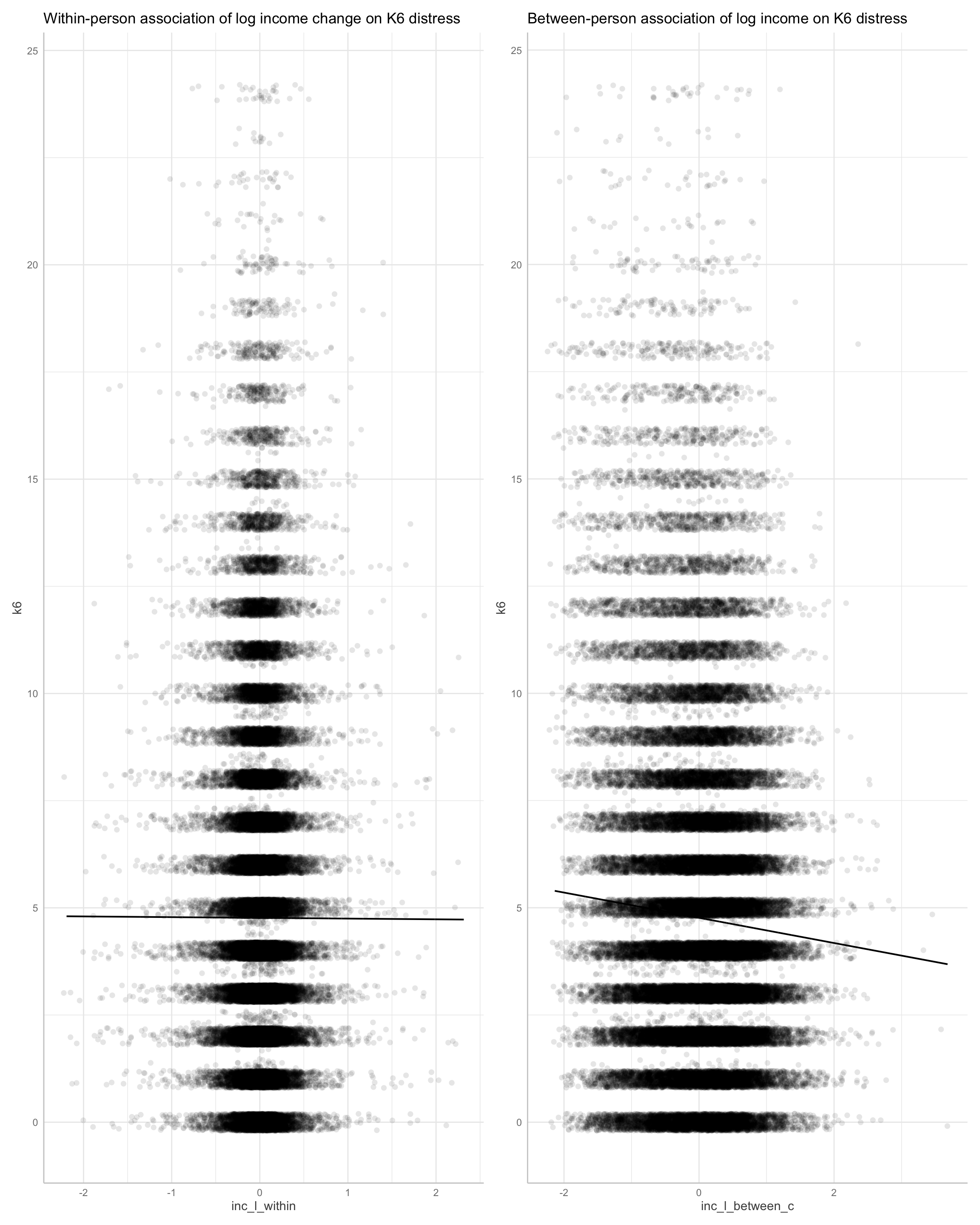
We find evidence for steep between person effects of income on k6.
GEE
Here we will used lagged values of the exposure to adjust for confounders and IP weights.
This result doesn’t make much sense.
Show code
str(dt)
'data.frame':   56714 obs. of  28 variables:
 $ id              : Factor w/ 67690 levels "1","2","3","4",..: 2 4 10 10 15 15 16 16 16 16 ...
 $ k6              : num  3 3 3 5 3 5 6 3 0 0 ...
 $ k6_lag          : num  2 3 3 10 4 3 1 6 3 0 ...
 $ inc_l_lag       : num  11.8 12.2 10.8 11.1 11.1 ...
 $ age_lag_lag     : num  37.6 38.8 45.9 49.4 41 ...
 $ eth_lag_lag     : Factor w/ 4 levels "Euro","Maori",..: 1 1 2 2 2 2 1 1 1 1 ...
 $ urban_lag_lag   : Factor w/ 2 levels "Not_Urban","Urban": 2 2 1 1 2 1 1 1 1 1 ...
 $ edu_lag_lag     : num  10 9 8 8 4 4 5 5 5 5 ...
 $ church_l_lag_lag: num  0 0 0 0 0 0 0 0 0 0 ...
 $ nzdep_lag_lag   : num  3 6 7 7 8 2 1 1 1 1 ...
 $ partner_lag_lag : num  0 1 0 0 1 1 1 1 1 1 ...
 $ emp_lag_lag     : num  2 2 2 2 1 2 2 1 1 1 ...
 $ male_lag_lag    : Factor w/ 2 levels "Not_Male","Male": 2 2 1 1 2 2 2 2 2 2 ...
 $ inc_l           : num  11.8 12.2 10.8 11.2 11.4 ...
 $ age_lag         : num  38.7 40.3 46.9 50.2 42 ...
 $ emp_lag         : num  2 2 2 2 1 1 1 1 1 1 ...
 $ partner_lag     : num  0 1 0 0 1 1 1 1 1 1 ...
 $ male_lag        : Factor w/ 2 levels "Not_Male","Male": 2 2 1 1 2 2 2 2 2 2 ...
 $ edu_lag         : num  10 9 8 8 4 4 5 5 5 5 ...
 $ eth_lag         : Factor w/ 4 levels "Euro","Maori",..: 1 1 2 2 2 2 1 1 1 1 ...
 $ church_l_lag    : num  0 0 0 0 0 0 0 0 0 0 ...
 $ urban_lag       : Factor w/ 2 levels "Not_Urban","Urban": 2 2 1 1 2 1 1 1 1 1 ...
 $ religious_lag   : num  1 1 1 1 1 1 1 1 1 1 ...
 $ nzdep_lag       : num  3 6 7 7 8 2 1 1 1 1 ...
 $ inc_l_lag_lag   : num  11.7 12.1 10.7 10.9 10.9 ...
 $ Id              : Factor w/ 67690 levels "1","2","3","4",..: 2 4 10 10 15 15 16 16 16 16 ...
 $ Wave            : Factor w/ 11 levels "2009","2010",..: 11 11 6 10 6 11 7 8 9 11 ...
 $ time            : num  0 0 0 4 0 5 0 1 2 4 ...
Show code
m2 <- geeglm(
  k6  ~
    inc_l +
    k6_lag +
    inc_l_lag +
    inc_l_lag_lag, #+
    # as.numeric(age_c_lag_lag) +
    # male_lag_lag +
    # eth_lag_lag +
    # emp_lag_lag +
    # nzdep_lag_lag +
    # partner_lag_lag+
    # urban_lag_lag,
  data = dt_weights_use_2,
  id = id,
  weights = ipw,
  waves = time,
  corstr = "ar1"
)

parameters::model_parameters(m2) %>%
  print_html()
| Model Summary | |||||
|---|---|---|---|---|---|
| Parameter | Coefficient | SE | 95% CI | Chi2(1) | p |
| (Intercept) | 2.06 | 0.15 | (1.75, 2.36) | 177.21 | < .001 |
| inc l | -0.12 | 0.03 | (-0.19, -0.06) | 12.77 | < .001 |
| k6 lag | 0.80 | 3.79e-03 | (0.79, 0.81) | 44614.72 | < .001 |
| inc l lag | 0.18 | 0.05 | (0.09, 0.27) | 14.34 | < .001 |
| inc l lag lag | -0.15 | 0.04 | (-0.22, -0.08) | 16.57 | < .001 |
Show code
If we remove weights the model makes sense.
Mixed effects approach: IPW
What if we were to use a mixed effects model?
Show code
library(gamm4)
library(splines)

# lmer
m2_lmer <- lmer(
  k6  ~
    k6_lag +
    inc_l +
    inc_l_lag +
    inc_l_lag_lag +
   (1  | id),
  data = dt_weights_use_2,
  weights = dt_weights_use_2$ipw
)

parameters::model_parameters(m2_lmer) %>%
  print_html()
| Model Summary | |||||
|---|---|---|---|---|---|
| Parameter | Coefficient | SE | 95% CI | t(56707) | p |
| Fixed Effects | |||||
| (Intercept) | 3.14 | 0.19 | (2.76, 3.51) | 16.36 | < .001 |
| k6 lag | 0.71 | 3.00e-03 | (0.71, 0.72) | 237.24 | < .001 |
| inc l | -0.12 | 0.03 | (-0.19, -0.06) | -4.01 | < .001 |
| inc l lag | 0.15 | 0.04 | (0.08, 0.22) | 4.15 | < .001 |
| inc l lag lag | -0.18 | 0.03 | (-0.24, -0.12) | -5.57 | < .001 |
| Random Effects | |||||
| SD (Intercept: id) | 0.00 | ||||
| SD (Residual) | 2.68 | ||||
Show code
We find support for an income effect.
Mixed effects approach (no IPW)
Show code
m2_lmer2 <- lmer(
  k6  ~   +
    k6_lag +
    inc_l +
    inc_l_lag  +
    inc_l_lag_lag +
    as.numeric(age_lag_lag) +
    male_lag_lag +
    eth_lag_lag +
    emp_lag_lag +
    nzdep_lag_lag +
    partner_lag_lag+
    urban_lag_lag + (1 + time|id),
  data = dt_weights_use_2
)


# we find an effect
parameters::model_parameters(m2_lmer2) %>%
  print_html()
| Model Summary | |||||
|---|---|---|---|---|---|
| Parameter | Coefficient | SE | 95% CI | t(56696) | p |
| Fixed Effects | |||||
| (Intercept) | 5.87 | 0.24 | (5.39, 6.35) | 24.06 | < .001 |
| k6 lag | 0.68 | 3.12e-03 | (0.68, 0.69) | 218.34 | < .001 |
| inc l | -0.21 | 0.03 | (-0.27, -0.15) | -6.67 | < .001 |
| inc l lag | 0.06 | 0.04 | (-7.68e-03, 0.14) | 1.75 | 0.080 |
| inc l lag lag | -0.10 | 0.03 | (-0.16, -0.03) | -2.99 | 0.003 |
| age lag lag | -0.03 | 9.46e-04 | (-0.03, -0.03) | -29.13 | < .001 |
| male lag lag (Male) | -4.35e-04 | 0.02 | (-0.05, 0.05) | -0.02 | 0.985 |
| eth lag lag (Maori) | -0.04 | 0.04 | (-0.12, 0.03) | -1.23 | 0.219 |
| eth lag lag (Pacific) | -2.56e-03 | 0.08 | (-0.16, 0.15) | -0.03 | 0.974 |
| eth lag lag (Asian) | 0.09 | 0.06 | (-0.04, 0.21) | 1.39 | 0.165 |
| emp lag lag | -0.16 | 0.03 | (-0.22, -0.10) | -5.16 | < .001 |
| nzdep lag lag | 0.02 | 4.44e-03 | (0.01, 0.03) | 5.06 | < .001 |
| partner lag lag | -0.06 | 0.03 | (-0.12, -7.65e-03) | -2.22 | 0.026 |
| urban lag lag (Urban) | 0.11 | 0.03 | (0.06, 0.16) | 4.25 | < .001 |
| Random Effects | |||||
| SD (Intercept: id) | 0.00 | ||||
| SD (time: id) | 2.45e-06 | ||||
| Cor (Intercept~time: id) | |||||
| SD (Residual) | 2.65 | ||||
Show code
Here we find support for a linear relationship.
Mixed effects models with splines
Finally, let us consider splines.
Show code
library(splines)

m2_lmer3 <- lmer(
  k6  ~    +
    bs(inc_l) +
     bs(inc_l_lag) +
     bs(inc_l_lag_lag) +
    as.numeric(age_lag_lag) +
    male_lag_lag +
    eth_lag_lag +
    emp_lag_lag +
    nzdep_lag_lag +
    partner_lag_lag+
    urban_lag_lag  + (1|id),
  data = dt_weights_use_2
)
# we find an effect
parameters::model_parameters(m2_lmer3) %>%
  print_html()
| Model Summary | |||||
|---|---|---|---|---|---|
| Parameter | Coefficient | SE | 95% CI | t(56693) | p |
| Fixed Effects | |||||
| (Intercept) | 11.07 | 0.22 | (10.63, 11.51) | 49.31 | < .001 |
| inc l (1st degree) | -0.69 | 0.40 | (-1.48, 0.10) | -1.71 | 0.087 |
| inc l (2nd degree) | -2.89 | 0.44 | (-3.76, -2.02) | -6.52 | < .001 |
| inc l (3rd degree) | 0.72 | 0.80 | (-0.85, 2.29) | 0.90 | 0.369 |
| inc l lag (1st degree) | -1.86 | 0.43 | (-2.71, -1.01) | -4.29 | < .001 |
| inc l lag (2nd degree) | 0.73 | 0.44 | (-0.13, 1.59) | 1.66 | 0.098 |
| inc l lag (3rd degree) | -2.65 | 0.79 | (-4.19, -1.11) | -3.36 | < .001 |
| inc l lag lag (1st degree) | -1.39 | 0.41 | (-2.19, -0.58) | -3.39 | < .001 |
| inc l lag lag (2nd degree) | -0.14 | 0.42 | (-0.96, 0.67) | -0.35 | 0.730 |
| inc l lag lag (3rd degree) | -2.08 | 0.74 | (-3.53, -0.63) | -2.82 | 0.005 |
| age lag lag | -0.07 | 1.82e-03 | (-0.08, -0.07) | -40.51 | < .001 |
| male lag lag (Male) | -0.05 | 0.05 | (-0.15, 0.05) | -1.07 | 0.286 |
| eth lag lag (Maori) | -0.02 | 0.07 | (-0.15, 0.11) | -0.25 | 0.804 |
| eth lag lag (Pacific) | 0.22 | 0.13 | (-0.04, 0.49) | 1.66 | 0.097 |
| eth lag lag (Asian) | 0.40 | 0.12 | (0.17, 0.64) | 3.36 | < .001 |
| emp lag lag | -0.10 | 0.04 | (-0.18, -0.03) | -2.58 | 0.010 |
| nzdep lag lag | 0.04 | 6.86e-03 | (0.03, 0.06) | 6.43 | < .001 |
| partner lag lag | -0.15 | 0.05 | (-0.24, -0.06) | -3.26 | 0.001 |
| urban lag lag (Urban) | 0.21 | 0.04 | (0.13, 0.28) | 5.56 | < .001 |
| Random Effects | |||||
| SD (Intercept: id) | 2.99 | ||||
| SD (Residual) | 2.11 | ||||
Show code
Error: Confidence intervals could not be computed.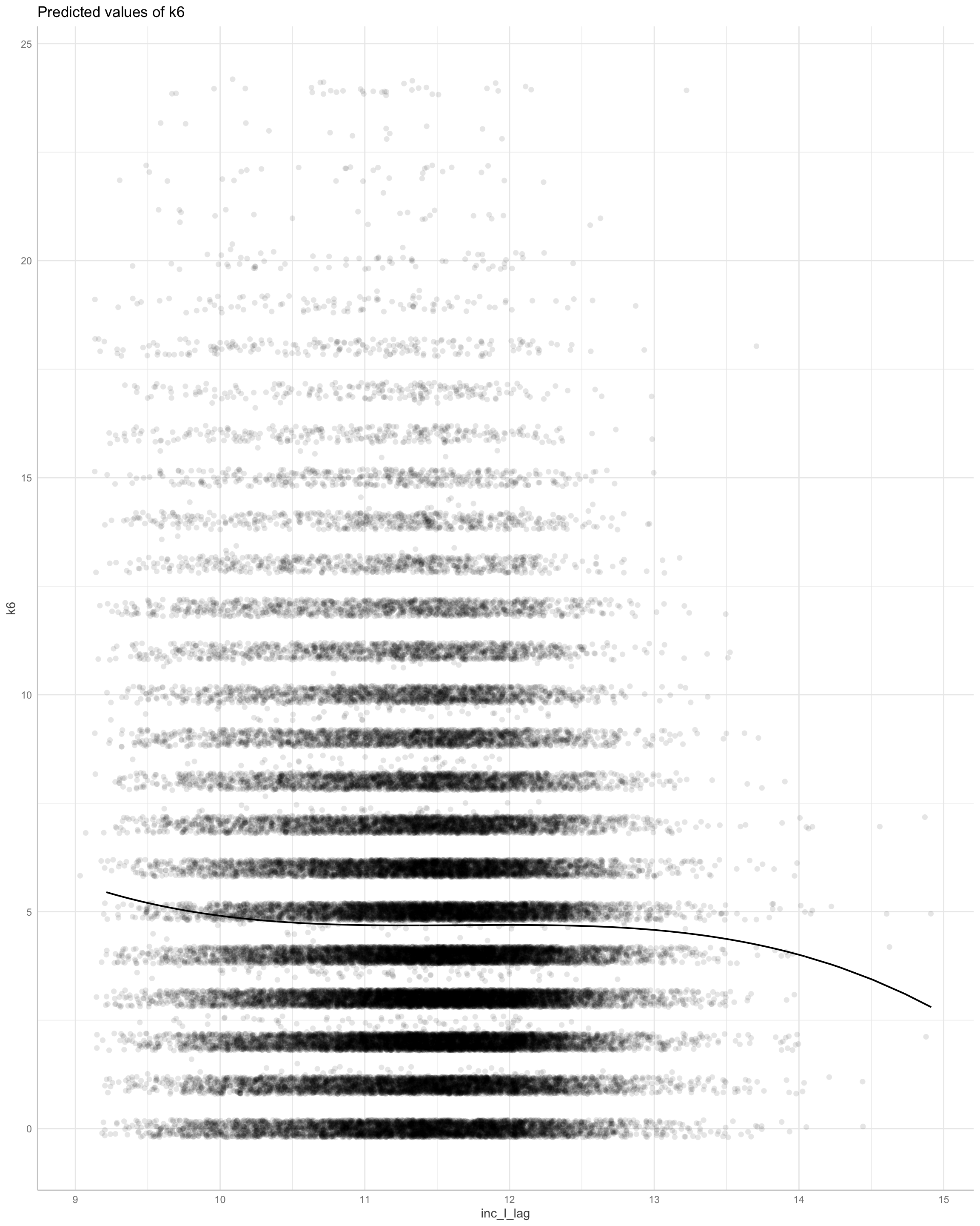
This suggests a linear decline in distress from income, at the high end of income.
We cannot obtain confidence intervales here. The linear model would appear sufficient. Greater income causes lower psychological distress.
Questions
Key points: - need to multiply impute - Use GEE - IP weighting = important, but does it makes sense for continuous exposures? - Model specification = important. - Handling of zero income? - Need to adjust for more confounders at the next iteration.
- Sensitivity tests.
G-estimation (just testing)
This is possibly not the right approach to our question. Notably, however, the model recovers a larger effect estimate.
We must handle attrition. There is likely to be selection on those who remain in the study. Note: the model below won’t run because time (k) needs to be ordered k…K+1 with no breaks.
Show code
# we do not evaluate this to save time

library(gesttools)
# must start at 1

dg <- df %>%
  dplyr::filter(YearMeasured == 1)  %>%
  dplyr::filter(Wave != 2009) %>% # no k6 measure
  dplyr::filter(
    !is.na(KESSLER6sum),
    !is.na(Household.INC),
    !is.na(EthnicCats),
    !is.na(Male),
    !is.na(Urban),
    !is.na(Employed)
  ) %>%
  dplyr::select(
    Id,
    Household.INC,
    KESSLER6sum,
    NZdep,
    Wave,
    # TSCORE,
    Age,
    # Religion.Prayer,
    #  Religion.Scripture,
    Religion.Church,
    Male,
    Edu,
    EthnicCats,
    Urban,
    Wave,
    Employed,
    Partner,
    Religious,
    Parent,
    NZdep,
    YearMeasured
  ) %>%
  dplyr::mutate(
    k6 = as.numeric(KESSLER6sum),
    age = (Age),
    inc_l = log(Household.INC + 1),
    emp = as.numeric(Employed),
    age_c = scale(Age, scale = F),
    employed = as.numeric(Employed) - 1,
    nzdep = as.numeric(NZdep),
    #  pray_l = log(Religion.Prayer + 1),
    #  script_l = log(Religion.Scripture + 1),
    church_l = log(Religion.Church + 1),
    edu = as.numeric(Edu),
    partner = as.numeric(Partner),
    male = as.numeric(Male),
    eth = EthnicCats,
    nzdep = as.numeric(NZdep),
    religious = as.numeric(Religious),
    urban = as.numeric(Urban),
    ym = as.numeric(YearMeasured) - 1
  ) %>%
  dplyr::group_by(Id) %>% filter(n() > 8) %>%
  ungroup() %>%
  arrange(Id, Wave)

# must start at 1
dg$time <- as.integer(dg$Wave) - 1
length(unique(dg$Id)) # 2366

dg1 <- dg %>%
  select(Id, time, inc_l, k6, male, urban, employed, nzdep, religious) %>%
  group_by(Id) %>%
  mutate(time = time - min(time) + 1) %>%
  mutate(mxtime = max(time)) %>%
  ungroup() %>%
  mutate(id = as.numeric(factor(Id))) %>%
  select(-Id) %>%
  drop_na()

dg2 <- as.data.frame(dg1)

head(dg2)
dgg <- FormatData(
  dg2,
  idvar = "id",
  timevar = "time",
  An = "inc_l",
  Cn = "mxtime",
  varying = c("k6", "inc_l", "employed", "religious", "nzdep", "urban", "male"),
  GenerateHistory = TRUE,
  GenerateHistoryMax = NA
)

head(dgg$k6)
head(dg1)
str(dgg


    test <- gestMultiple(
      dgg,
      idvar = "id",
      timevar = "time",
      Yn = "k6",
      An = "inc_l",
      Ybin = FALSE,
      Abin = FALSE,
      Acat = FALSE,
      Lny = c("employed", "religious", "nzdep", "urban", "male"),
      Lnp = c("employed", "religious", "nzdep", "urban", "male"),
      type = 1 #,
      # Cn = "mxtime",
      # LnC =c("employed", "religious", "nzdep", "urban", "male"),
      # cutoff = "mxtime"
    )
    summary(test$psi)


    #
    test2 <- gestboot(
      gestMultiple,
      dgg,
      idvar = "id",
      timevar = "time",
      Yn = "k6",
      An = "inc_l",
      Ybin = FALSE,
      Abin = FALSE,
      Acat = FALSE,
      Lny = c("employed", "religious", "nzdep", "urban", "male"),
      Lnp = c("employed", "religious", "nzdep", "urban", "male"),
      type = 1 ,
      #,
      alpha = .05,
      bn = 5,
      oneside = "twosided",
      seed = 123
    )
    # Cn = "mxtime",
    # LnC =c("employed", "religious", "nzdep", "urban", "male"),
    # cutoff = "mxtime"

#saveRDS(test2, here::here("models", "test2"))$original
inc_l
-0.1703885
$mean.boot
inc_l
-0.1746761
$conf
2.5% 97.5%
inc_l -0.2138265 -0.1554299
$conf.Bonferroni
2.5% 97.5%
inc_l -0.2138265 -0.1554299
$boot.results
# A tibble: 5 × 1
inc_l
<dbl>
1 -0.169
2 -0.170
3 -0.155
4 -0.219
5 -0.161
attr(,"class")
[1] "Results"Gformula
Experimental
Show code
dgf <- df %>%
 dplyr::filter(Wave != 2009) %>% # no k6 measure
  droplevels() %>%
 dplyr::filter(YearMeasured == 1)  %>%
  dplyr::select(
    Id,
    Household.INC,
    KESSLER6sum,
    NZdep,
    Wave,
   # TSCORE,
    Age,
    Euro,
  # Religion.Prayer,
  #  Religion.Scripture,
    Religion.Church,
    Male,
    Edu,
    EthnicCats,
    Urban,
    Wave,
    Employed,
    Partner,
    Religious,
    Parent,
    NZdep,
   YearMeasured
  ) %>%
  dplyr::mutate(
    wave = as.numeric(Wave) -1,
    k6 = as.numeric(KESSLER6sum),
    age = (Age),
    inc_l = log(Household.INC + 1),
    emp = as.numeric(Employed)-1,
    euro = as.numeric(Euro)-1,
    age_c = scale(Age, scale = F),
    employed = as.numeric(Employed)-1,
    nzdep = as.numeric(NZdep),
  #  pray_l = log(Religion.Prayer + 1),
  #  script_l = log(Religion.Scripture + 1),
    church_l = log(Religion.Church + 1),
    edu = as.numeric(Edu),
    partner = as.numeric(Partner),
    male = as.numeric(Male)-1,
    eth = EthnicCats,
    nzdep = as.numeric(NZdep),
    religious=as.numeric(Religious)-1,
    urban = as.numeric(Urban)-1) %>%
    dplyr::group_by(Id) %>%
  select(Id, k6,  inc_l, age, wave, euro, employed, nzdep, partner, male, religious, urban) %>%
  #mutate_all(~as.numeric(.)) %>%
 # drop_na() %>%
  filter(n() == 10) %>%
  ungroup() %>%
  mutate(time = wave - min(wave))%>%
  mutate(mxtime = max(time))%>%
  mutate(id = as.numeric(factor(Id)))%>%
  mutate(k6_s = scale(k6)) %>%
  arrange(id,time)

max(dgf$id)
[1] 1441Show code
library(gfoRmula)

#This isn't working

# "Error in error_catch(id = id, nsimul = nsimul, intvars = intvars, interventions = interventions,  :
# Time variable in obs_data not correctly specified. For each individual time records should begin with 0 (or, optionally -i if using i lags) and increase in increments of 1, where no time records are skipped."
dgf<- dgf%>%
rename(t0= time,
       A = partner,
       L1 = "inc_l",
       Y = "k6_s")
dgf
id <- 'id'
time_name <- 't0'
time_points <-10
covnames <- c(
    "L1",
    "A"
  )
outcome_name <- 'Y'
outcome_type <- 'continuous_eof'
covtypes =  c(
    "normal", "binary"
  )

intvars <- list('A', 'A')

interventions <- list(list(c(static, rep(0, 10))),
                      list(c(static, rep(1, 10))))

int_descript <- c('Never treat', 'Always treat')

histories <- list(lagged)

histvars = list(c("L1", "A"))

covparams <- list(
    covmodels = c(
      L1 ~ lag1_A   +  t0,
      A ~ lag1_A + L1  + t0))
covnames

ymodel <- Y ~  L1 + lag1_A + lag1_L1 + t0

library(data.table)
dgf<- data.table(dgf)

test3 <- gformula(
  obs_data = dgf,
  id = id,
  time_name = time_name,
  time_points = time_points,
  covnames = covnames,
  outcome_name = outcome_name,
  outcome_type = outcome_type,
  covtypes = covtypes,
  covparams = covparams,
  ymodel = ymodel,
  intvars = intvars,
  interventions = interventions,
  int_descript = int_descript,
  histories = histories,
  histvars = histvars,
  #basecovs = c("male","euro"),
  nsimul = 10000,
  seed = 1234)
plot(test3)
Show code
id <- 'id'
time_points <- 7
time_name <- 't0'
covnames <- c('L1', 'L2', 'A')
outcome_name <- 'Y'
outcome_type <- 'survival'
covtypes <- c('binary', 'bounded normal', 'binary')
histories <- c(lagged, lagavg)
histvars <- list(c('A', 'L1', 'L2'), c('L1', 'L2'))
covparams <- list(covmodels = c(L1 ~ lag1_A + lag_cumavg1_L1 + lag_cumavg1_L2 +
                                  L3 + t0,
                                L2 ~ lag1_A + L1 + lag_cumavg1_L1 +
                                  lag_cumavg1_L2 + L3 + t0,
                                A ~ lag1_A + L1 + L2 + lag_cumavg1_L1 +
                                  lag_cumavg1_L2 + L3 + t0))
ymodel <- Y ~ A + L1 + L2 + L3 + lag1_A + lag1_L1 + lag1_L2 + t0
intvars <- list('A', 'A')
interventions <- list(list(c(static, rep(0, time_points))),
                      list(c(static, rep(1, time_points))))
int_descript <- c('Never treat', 'Always treat')
nsimul <- 10000

gform_basic <- gformula(obs_data = basicdata_nocomp, id = id,
                        time_points = time_points,
                        time_name = time_name, covnames = covnames,
                        outcome_name = outcome_name,
                        outcome_type = outcome_type, covtypes = covtypes,
                        covparams = covparams, ymodel = ymodel,
                        intvars = intvars,
                        interventions = interventions,
                        int_descript = int_descript,
                        histories = histories, histvars = histvars,
                        basecovs = c('L3'), nsimul = nsimul,
                        seed = 1234)

plot(gform_basic)
Gformulate Church attendance and distress
Prepare data
Show code
dgf <- df %>%
  dplyr::filter(YearMeasured == 1)  %>%
  dplyr::filter(Wave != 2009) %>% # no k6 measure
  dplyr::filter(!is.na(KESSLER6sum), !is.na(Religion.Church)) %>%
  dplyr::group_by(Id) %>% filter(n() > 9) %>%
  ungroup() %>%
  dplyr::mutate(inc_quant = ntile(Household.INC, 4)-1) %>% # income categories
  dplyr::mutate(k6_cats = cut(
    KESSLER6sum,
    breaks = c(-Inf, 5, 13, Inf),
    # create Kessler 6 diagnostic categories
    labels = c("Low Distress", "Moderate Distress", "Serious Distress"),
    right = TRUE
  )) %>%
    dplyr::mutate(k6_bin = cut(
    KESSLER6sum,
    breaks = c(-Inf, 13, Inf),
    # create Kessler 6 diagnostic categories
    labels = c("Low Distress",  "Serious Distress"),
    right = TRUE
  )) %>%
  dplyr::mutate(church_ord = cut(
    Religion.Church,
    breaks = c(-Inf, 0, 1, 3, Inf),
    labels = c("0", "1", "1-3", "4-up"),
    right = TRUE
  )) %>%
    dplyr::mutate(church_bin  = cut(
    Religion.Church,
    breaks = c(-Inf, 0,  Inf),
    labels = c("0", "some"),
    right = TRUE
  )) %>%
  dplyr::mutate(k6 =  as.numeric(KESSLER6sum) ) %>%
  dplyr::mutate(church_bin =  as.numeric(church_bin) - 1) %>%
  dplyr::select(Id,
                inc_quant,
                church_ord,
                church_bin,
                k6,
                k6_bin,
                k6_cats,
                Wave,
                GenCohort,
                Euro,
                Religious,
                Male,
                Urban,
                Employed,
                Household.INC,
                Partner,
                Wave) %>%
  mutate(time0 = as.numeric(Wave)) %>%
  mutate(time = time0 - min(time0)) %>%
  dplyr::mutate(across(
    c(inc_quant,
      k6,
      church_ord,
      church_bin,
      k6_cats,
      Employed,
      Religious,
      Urban,
      Partner),
    list(lag = lag)
  )) %>%
  drop_na() %>%
    dplyr::group_by(Id) %>% filter(n() > 9) %>%
    filter(n() == 10) %>%
  dplyr::arrange(Id, Wave) %>%
   dplyr::group_by(Id)%>%
  mutate(time = (as.numeric(Wave) - min(as.numeric(Wave))) ) %>% # zero time is start for each person
   dplyr::ungroup(Id) %>%
   dplyr::mutate( Partner = as.numeric(Partner),
                  Male = as.numeric(Male),
                  GenCohort = as.numeric(GenCohort))

head(dgf$time)
[1] 0 1 2 3 4 5Show code
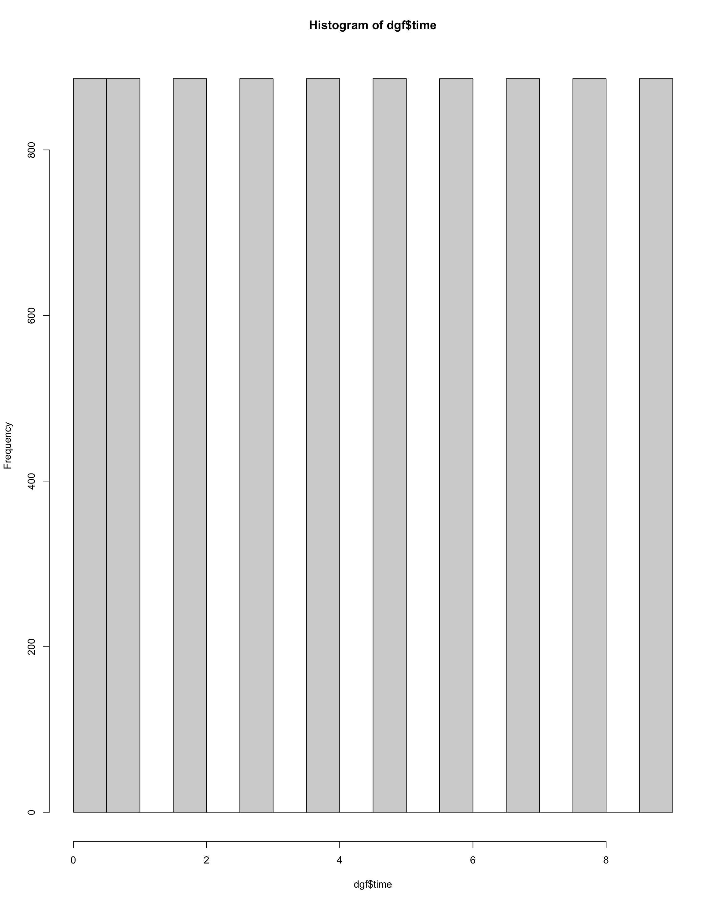
summary((dgf$time))
   Min. 1st Qu.  Median    Mean 3rd Qu.    Max.
    0.0     2.0     4.5     4.5     7.0     9.0
Show code
hist(dgf$time)
Show code
str(dgf)
tibble [8,860 × 27] (S3: tbl_df/tbl/data.frame)
 $ Id            : Factor w/ 67690 levels "1","2","3","4",..: 19 19 19 19 19 19 19 19 19 19 ...
 $ inc_quant     : num [1:8860] 0 0 0 0 0 0 0 0 0 0 ...
 $ church_ord    : Factor w/ 4 levels "0","1","1-3",..: 1 1 1 1 1 1 1 1 1 1 ...
 $ church_bin    : num [1:8860] 0 0 0 0 0 0 0 0 0 0 ...
 $ k6            : num [1:8860] 1 2 2 1 1 1 2 3 1 1 ...
 $ k6_bin        : Factor w/ 2 levels "Low Distress",..: 1 1 1 1 1 1 1 1 1 1 ...
 $ k6_cats       : Factor w/ 3 levels "Low Distress",..: 1 1 1 1 1 1 1 1 1 1 ...
 $ Wave          : Factor w/ 11 levels "2009","2010",..: 2 3 4 5 6 7 8 9 10 11 ...
 $ GenCohort     : num [1:8860] 1 1 1 1 1 1 1 1 1 1 ...
 $ Euro          : num [1:8860] 1 1 1 1 1 1 1 1 1 1 ...
 $ Religious     : Factor w/ 2 levels "Not_Religious",..: 2 1 2 2 2 2 1 1 2 2 ...
 $ Male          : num [1:8860] 1 1 1 1 1 1 1 1 1 1 ...
 $ Urban         : Factor w/ 2 levels "Not_Urban","Urban": 2 2 2 2 2 2 2 2 2 2 ...
 $ Employed      : Factor w/ 2 levels "0","1": 1 1 1 1 1 1 1 1 1 1 ...
 $ Household.INC : num [1:8860] 40000 40000 40000 40000 40000 40000 40000 40000 36000 36000 ...
 $ Partner       : num [1:8860] 1 1 1 1 1 1 1 1 1 1 ...
 $ time0         : num [1:8860] 2 3 4 5 6 7 8 9 10 11 ...
 $ time          : num [1:8860] 0 1 2 3 4 5 6 7 8 9 ...
 $ inc_quant_lag : num [1:8860] 1 0 0 0 0 0 0 0 0 0 ...
 $ k6_lag        : num [1:8860] 5 1 2 2 1 1 1 2 3 1 ...
 $ church_ord_lag: Factor w/ 4 levels "0","1","1-3",..: 1 1 1 1 1 1 1 1 1 1 ...
 $ church_bin_lag: num [1:8860] 0 0 0 0 0 0 0 0 0 0 ...
 $ k6_cats_lag   : Factor w/ 3 levels "Low Distress",..: 1 1 1 1 1 1 1 1 1 1 ...
 $ Employed_lag  : Factor w/ 2 levels "0","1": 2 1 1 1 1 1 1 1 1 1 ...
 $ Religious_lag : Factor w/ 2 levels "Not_Religious",..: 1 2 1 2 2 2 2 1 1 2 ...
 $ Urban_lag     : Factor w/ 2 levels "Not_Urban","Urban": 1 2 2 2 2 2 2 2 2 2 ...
$ Partner_lag : num [1:8860] 1 1 1 1 1 1 1 1 1 1 ...[1] 886Show code
library(data.table)
dgf <- data.table(dgf)
Show code
# not running


head(dgf)
id <- 'Id'
time_points <- 10
time_name <- 'time'
covnames <- c('Partner', 'Employed', 'church_bin')
outcome_name <- 'k6'
outcome_type <- 'continuous_eof'
covtypes <- c('binary', 'binary', 'binary')
histories <- c(lagged)
histvars <- list(c('church_bin', 'Partner', 'Employed'))
covparams <- list(covmodels = c(Partner ~  lag1_Partner + lag1_church_bin + time,
                                  Employed ~   lag1_Employed + Male + time,
                                  church_bin ~ lag1_church_bin  + GenCohort  + Male +  time))
ymodel <- k6 ~ church_bin + lag1_church_bin + Partner + Employed  + GenCohort + lag1_Partner + lag1_Employed
intvars <- list('church_bin', 'church_bin')
interventions <- list(list(c(static, rep(0, time_points))),
                        list(c(static, rep(1, time_points))))

int_descript <- c('Never treat', 'Threshold - lower bound 1')
nsimul <- 10000


# dgf%>%
#   group_by(Id) %>%
#   summarise(n = n()) %>%
#   count(n == 10)

gform_basic <- gformula(obs_data = dgf,
                        id = id,
                        time_points = time_points,
                        time_name = time_name,
                        covnames = covnames,
                        outcome_name = outcome_name,
                        outcome_type = outcome_type,
                        covtypes = covtypes,
                        covparams = covparams,
                        ymodel = ymodel,
                        intvars = intvars,
                        interventions = interventions,
                        int_descript = int_descript,
                        histories = histories,
                        histvars = histvars,
                        basecovs = c("Male","GenCohort"),
                        nsimul = nsimul,
                        seed = 1234)

plot(gform_basic)
Model
Show code
dg_gf <- ipw::ipwtm(
  exposure = church_bin,
  family = "binomial",
  link = "probit",
  type = "first",
  corstr = "ar1",
  id = "Id",
  timevar = "time",
  numerator = ~
     church_bin_lag  +
     GenCohort +
     Male +
     Euro +
   #  Partner +
    # Partner_lag +
     Employed +
     Employed_lag, #+
  denominator = ~ # lag treatment + lag outcome +  confounders +
     church_bin_lag  +
     k6_lag + # lag treatment + time invariant confounders
     GenCohort +
     Male +
     Euro +
     Partner +
     Partner_lag +
     Employed +
     Employed_lag,
  data = as.data.frame(dgf)
)


hist(dg_gf$ipw.weights)
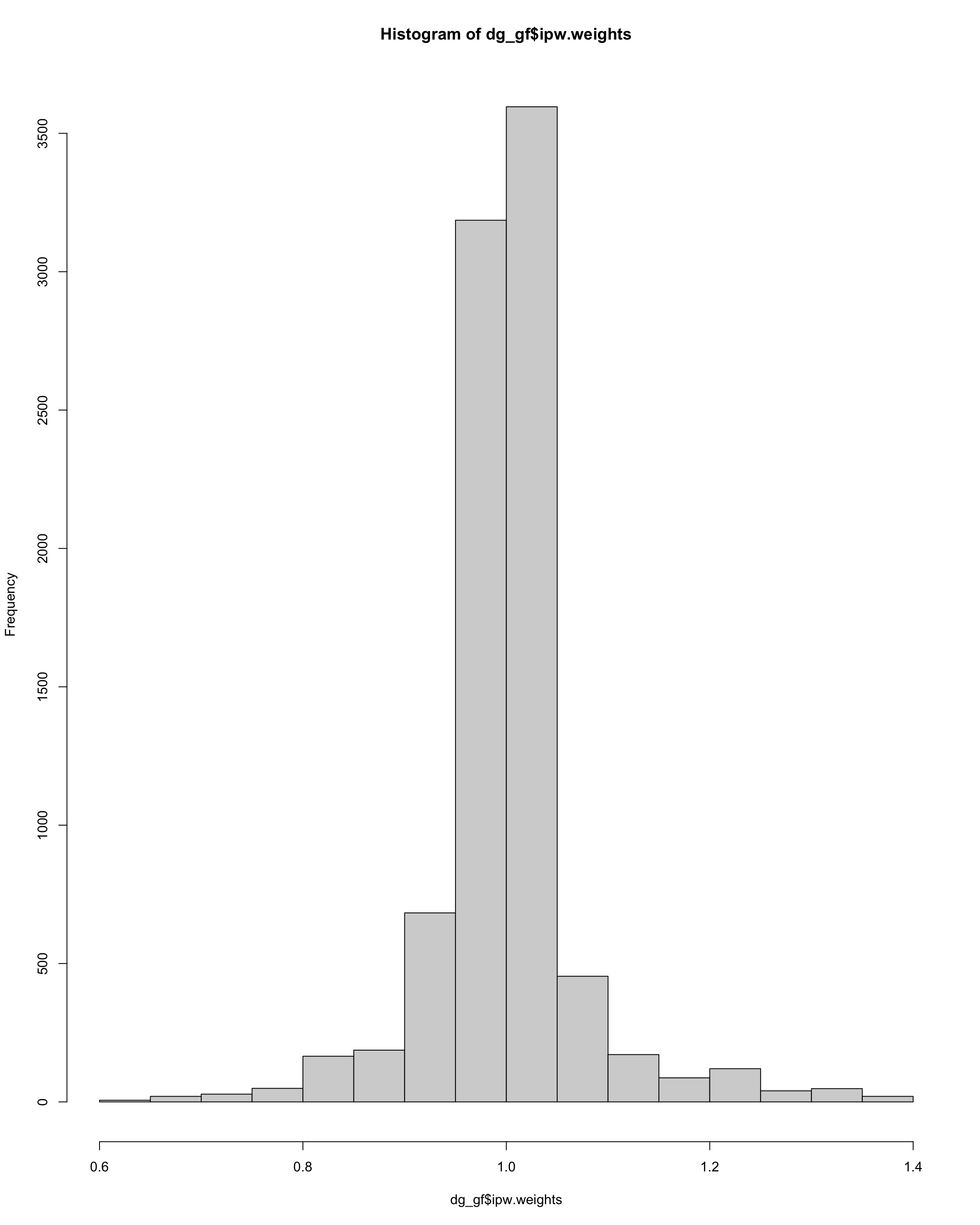
Show code
sum(dg_gf$ipw.weights > 10)
[1] 0Show code
## GEE
m0 <- geeglm(
k6 ~
church_bin +
church_bin_lag,
data = cdat,
id = Id,
family = "gaussian",
weights = ipw,
waves = time,
corstr = "ar1"
)
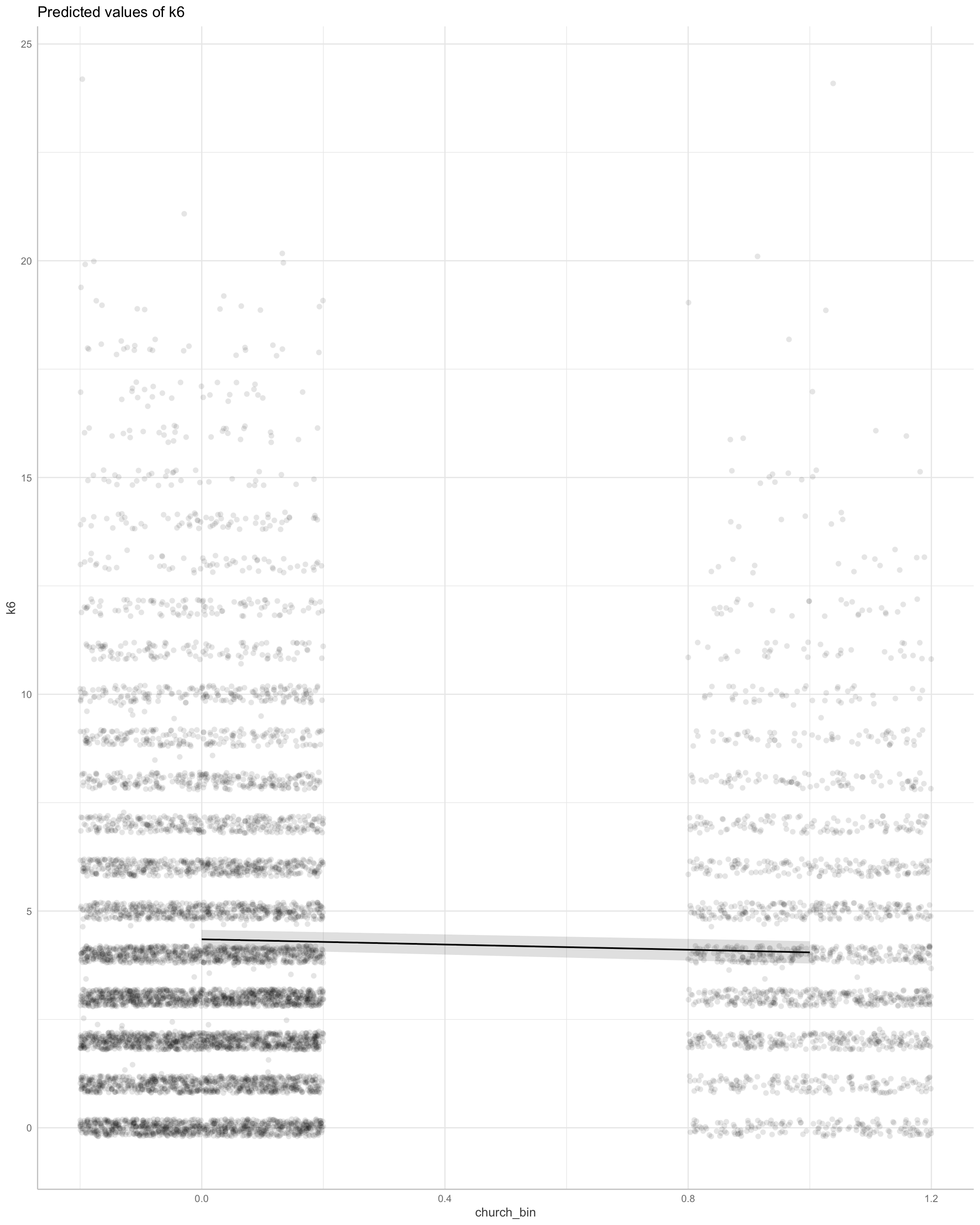
parameters::model_parameters(m0) %>%
print_html()
| Model Summary | |||||
|---|---|---|---|---|---|
| Parameter | Coefficient | SE | 95% CI | Chi2(1) | p |
| (Intercept) | 4.31 | 0.11 | (4.09, 4.53) | 1437.38 | < .001 |
| church bin | -0.30 | 0.12 | (-0.54, -0.07) | 6.41 | 0.011 |
| church bin lag | 0.19 | 0.12 | (-0.05, 0.42) | 2.48 | 0.115 |
Show code
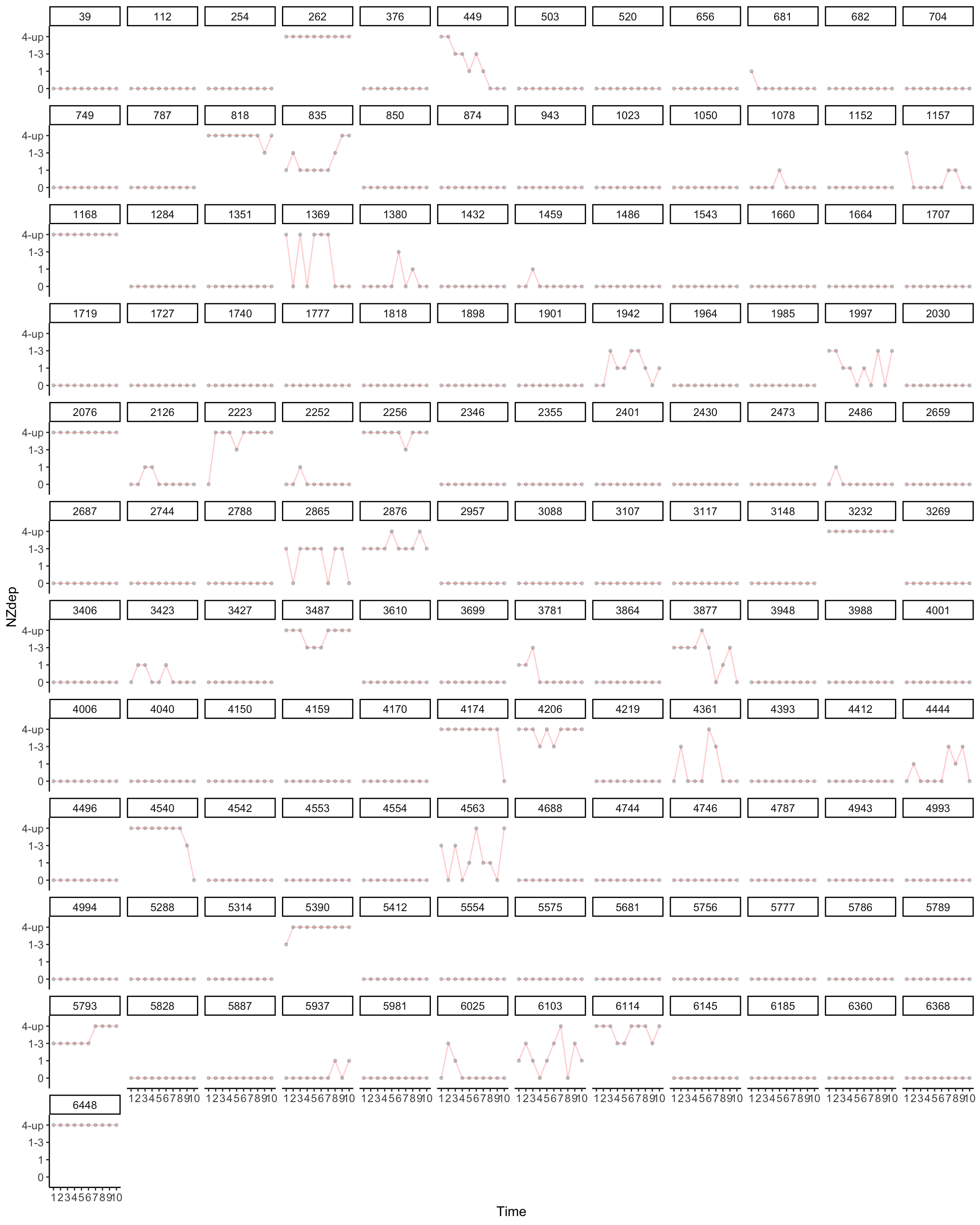
Change in church
Ordinal
Show code
widelong <-  dgf %>%
  dplyr::select(Id, church_ord, Wave) #

wide <- spread(widelong, Wave, church_ord)


wide2 <- wide[complete.cases(wide),]


x_var_list <- names(wide2[, 2:11])


wide2 <- as.data.frame(wide2)

plot_trajectories(
  data = wide2,
  id_var = "Id",
  var_list = x_var_list,
  line_colour = "red",
  xlab = "Time",
  ylab = "NZdep",
  connect_missing = F,
  scale_x_num = T,
  scale_x_num_start = 1,
  random_sample_frac = 0.15,
  seed = 1234
  #title_n = T
)  +
  facet_wrap( ~ Id)
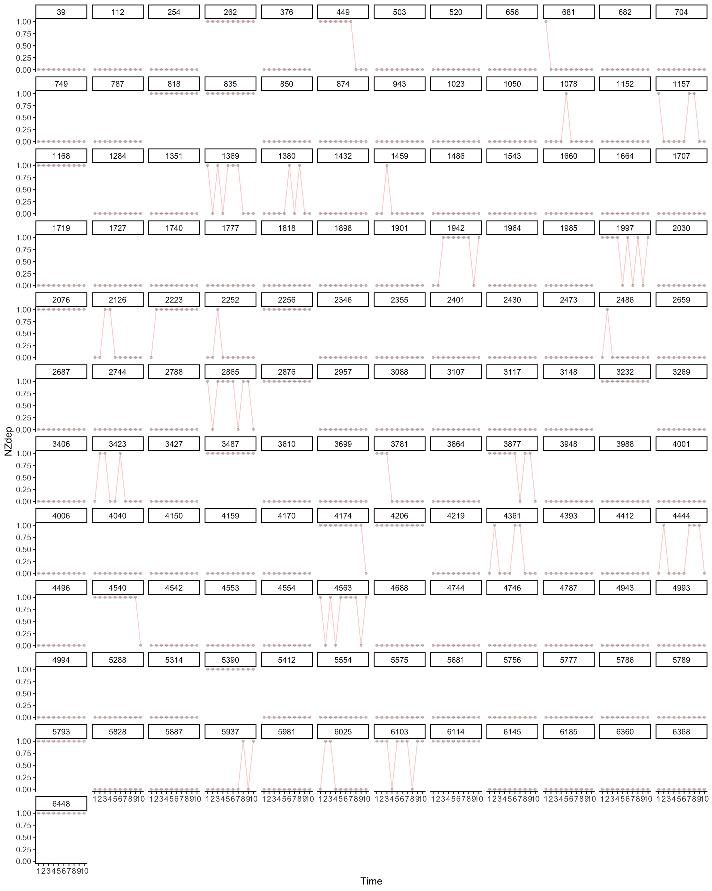
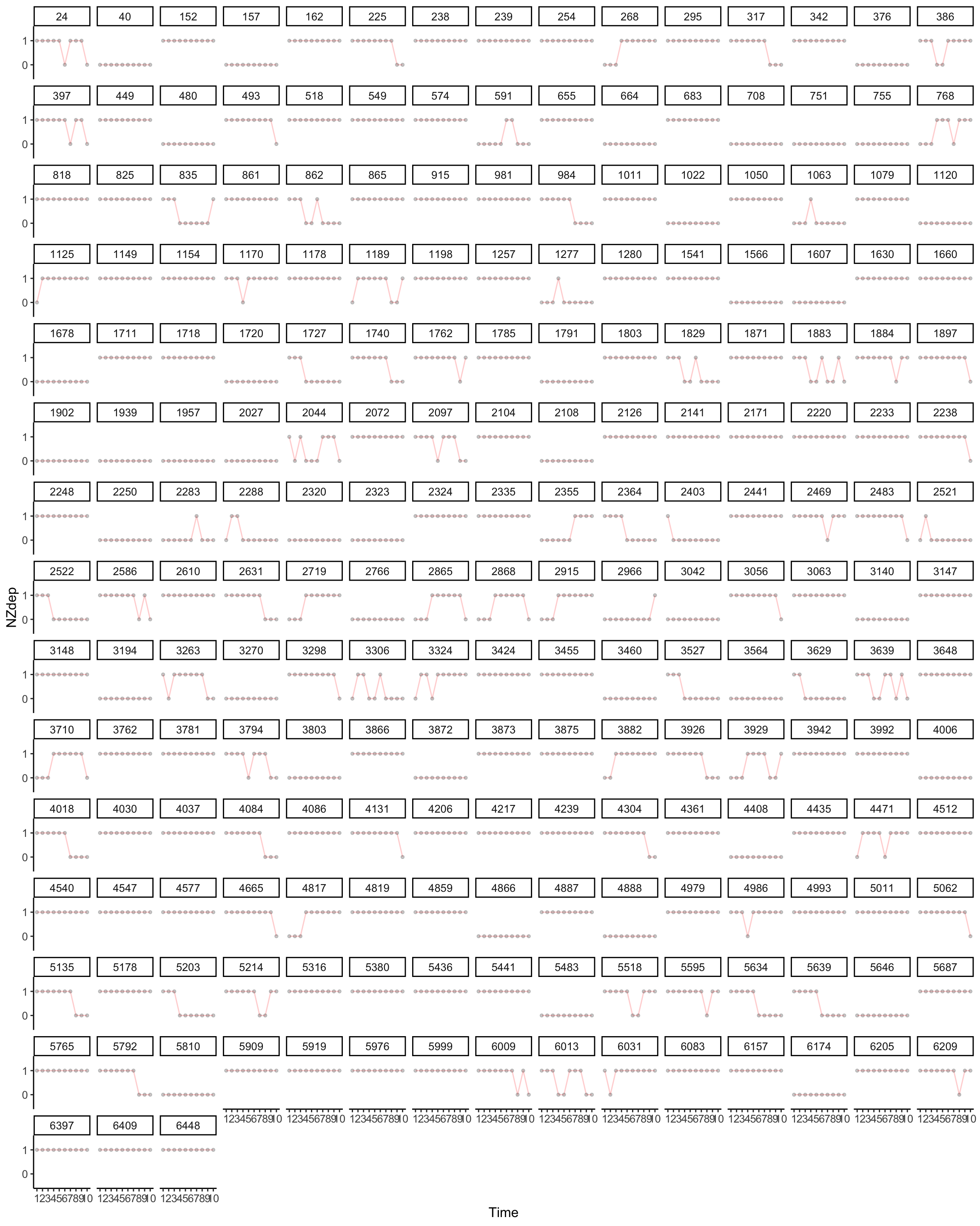
Binary church
Show code
widelong <-  dgf %>%
  dplyr::select(Id, church_bin, Wave) #

wide <- spread(widelong, Wave, church_bin)


wide2 <- wide[complete.cases(wide),]


x_var_list <- names(wide2[, 2:11])


wide2 <- as.data.frame(wide2)

plot_trajectories(
  data = wide2,
  id_var = "Id",
  var_list = x_var_list,
  line_colour = "red",
  xlab = "Time",
  ylab = "NZdep",
  connect_missing = F,
  scale_x_num = T,
  scale_x_num_start = 1,
  random_sample_frac = 0.15,
  seed = 1234
  #title_n = T
)  +
  facet_wrap( ~ Id)
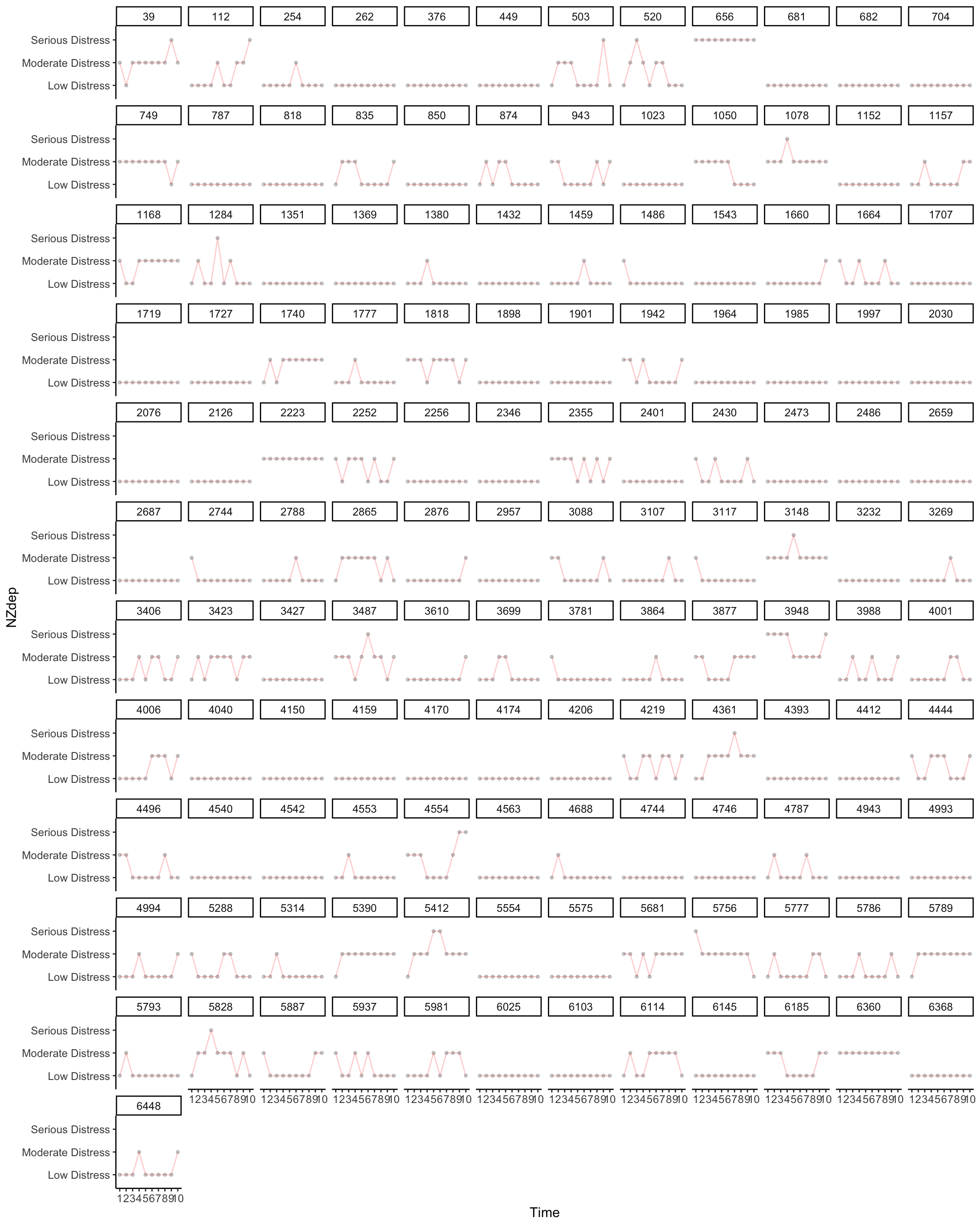
Change in K6
Show code
widelong <-  dgf %>%
  dplyr::select(Id, k6_cats, Wave) # x

wide <- spread(widelong, Wave, k6_cats)


wide2 <- wide[complete.cases(wide),]


x_var_list <- names(wide2[, 2:11])


wide2 <- as.data.frame(wide2)

plot_trajectories(
  data = wide2,
  id_var = "Id",
  var_list = x_var_list,
  line_colour = "red",
  xlab = "Time",
  ylab = "NZdep",
  connect_missing = F,
  scale_x_num = T,
  scale_x_num_start = 1,
  random_sample_frac = 0.15,
  seed = 1234
  #title_n = T
)  +
  facet_wrap( ~ Id)
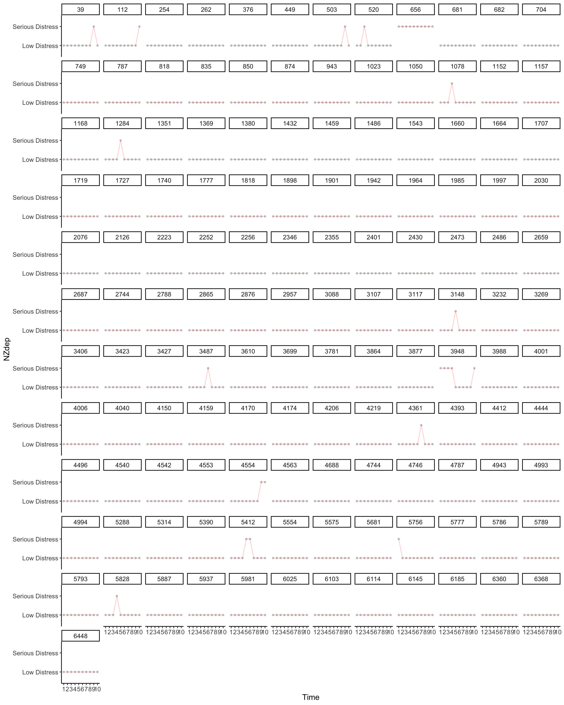
Binary k6
Show code
widelong <-  dgf %>%
  dplyr::select(Id, k6_bin, Wave) #

wide <- spread(widelong, Wave, k6_bin)


wide2 <- wide[complete.cases(wide),]


x_var_list <- names(wide2[, 2:11])


wide2 <- as.data.frame(wide2)

plot_trajectories(
  data = wide2,
  id_var = "Id",
  var_list = x_var_list,
  line_colour = "red",
  xlab = "Time",
  ylab = "NZdep",
  connect_missing = F,
  scale_x_num = T,
  scale_x_num_start = 1,
  random_sample_frac = 0.15,
  seed = 1234
  #title_n = T
)  +
  facet_wrap( ~ Id)
Ethnicity Change
Show code
# A tibble: 6 × 12
  Id    `2009` `2010` `2011` `2012` `2013` `2014` `2015`
  <fct> <fct>  <fct>  <fct>  <fct>  <fct>  <fct>  <fct>
1 2     Euro   <NA>   <NA>   <NA>   Euro   Euro   Euro
2 10    Maori  Maori  Maori  Maori  Maori  Maori  Maori
3 14    Euro   Euro   Euro   <NA>   Euro   Euro   Euro
4 15    Maori  Maori  Maori  Maori  Maori  Maori  Maori
5 16    Euro   Euro   Euro   Euro   Euro   Euro   Euro
6 18    Euro   <NA>   <NA>   Euro   Euro   Euro   Euro
# … with 4 more variables: `2016` <fct>, `2017` <fct>,
#   `2018` <fct>, `2019` <fct>
Show code
x_var_list <- names(wide2[, 2:11])


wide2 <- as.data.frame(wide2)

plot_trajectories(
  data = wide2,
  id_var = "Id",
  var_list = x_var_list,
  line_colour = "red",
  xlab = "Time",
  ylab = "NZdep",
  connect_missing = F,
  scale_x_num = T,
  scale_x_num_start = 1,
  random_sample_frac = 0.15,
  seed = 1234
  #title_n = T
)  +
  facet_wrap( ~ Id)
Employed change
Show code
# A tibble: 6 × 12
  Id    `2009` `2010` `2011` `2012` `2013` `2014` `2015`
  <fct> <fct>  <fct>  <fct>  <fct>  <fct>  <fct>  <fct>
1 2     1      <NA>   <NA>   <NA>   1      1      1
2 10    1      1      1      1      1      1      1
3 14    1      0      1      1      1      1      1
4 15    1      1      1      0      0      1      1
5 16    1      1      1      1      1      0      0
6 18    0      <NA>   <NA>   1      1      1      1
# … with 4 more variables: `2016` <fct>, `2017` <fct>,
#   `2018` <fct>, `2019` <fct>
Show code
x_var_list <- names(wide2[, 2:11])


wide2 <- as.data.frame(wide2)

plot_trajectories(
  data = wide2,
  id_var = "Id",
  var_list = x_var_list,
  line_colour = "red",
  xlab = "Time",
  ylab = "NZdep",
  connect_missing = F,
  scale_x_num = T,
  scale_x_num_start = 1,
  random_sample_frac = 0.15,
  seed = 1234
  #title_n = T
)  +
  facet_wrap( ~ Id)
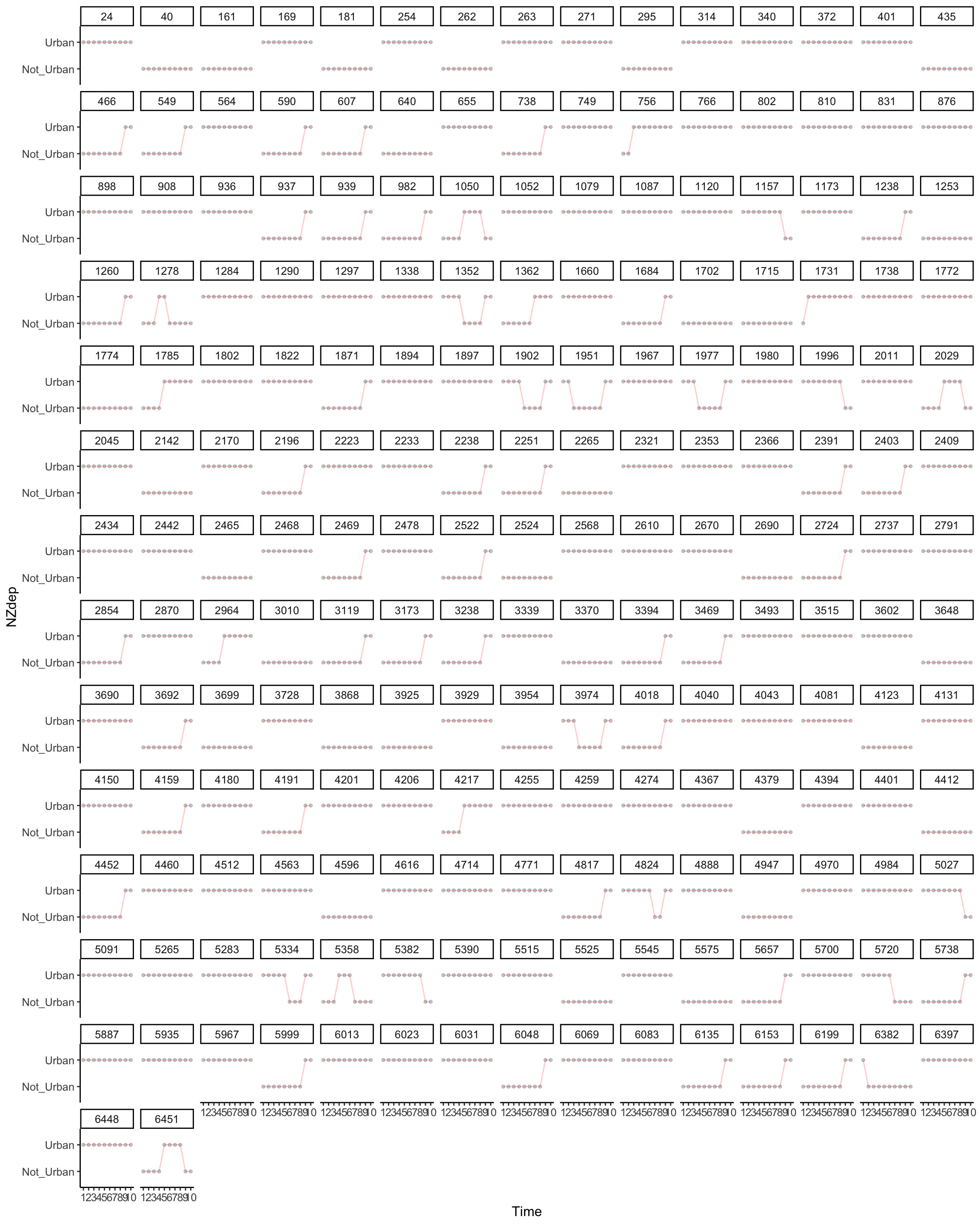
Urban change
Show code
# A tibble: 6 × 12
  Id    `2009`    `2010`  `2011` `2012` `2013` `2014` `2015`
  <fct> <fct>     <fct>   <fct>  <fct>  <fct>  <fct>  <fct>
1 2     <NA>      <NA>    <NA>   <NA>   Urban  Urban  Urban
2 10    Not_Urban Not_Ur… Not_U… Not_U… Not_U… Not_U… Not_U…
3 14    Urban     Urban   Urban  Urban  Urban  Urban  Urban
4 15    Urban     Urban   Urban  Urban  Urban  Urban  Not_U…
5 16    Urban     Urban   Urban  Urban  Not_U… Not_U… Not_U…
6 18    Urban     <NA>    <NA>   Urban  Urban  Urban  Urban
# … with 4 more variables: `2016` <fct>, `2017` <fct>,
#   `2018` <fct>, `2019` <fct>
Show code
x_var_list <- names(wide2[, 2:11])


wide2 <- as.data.frame(wide2)

plot_trajectories(
  data = wide2,
  id_var = "Id",
  var_list = x_var_list,
  line_colour = "red",
  xlab = "Time",
  ylab = "NZdep",
  connect_missing = F,
  scale_x_num = T,
  scale_x_num_start = 1,
  random_sample_frac = 0.15,
  seed = 1234
  #title_n = T
)  +
  facet_wrap( ~ Id)
Edu change
Show code
# A tibble: 6 × 10
  Id    `2009` `2012` `2013` `2014` `2015` `2016` `2017`
  <fct> <fct>  <fct>  <fct>  <fct>  <fct>  <fct>  <fct>
1 2     9      <NA>   9      9      9      9      9
2 10    7      7      7      7      7      7      <NA>
3 14    7      7      7      7      7      7      7
4 15    3      3      3      3      3      3      3
5 16    4      4      4      4      4      4      4
6 18    5      5      5      5      5      5      5
# … with 2 more variables: `2018` <fct>, `2019` <fct>
Show code
x_var_list <- names(wide2[, 2:9])


wide2 <- as.data.frame(wide2)

plot_trajectories(
  data = wide2,
  id_var = "Id",
  var_list = x_var_list,
  line_colour = "red",
  xlab = "Time",
  ylab = "NZdep",
  connect_missing = F,
  scale_x_num = T,
  scale_x_num_start = 1,
  random_sample_frac = 0.15,
  seed = 1234
  #title_n = T
)  +
  facet_wrap( ~ Id)
BMI - Checks
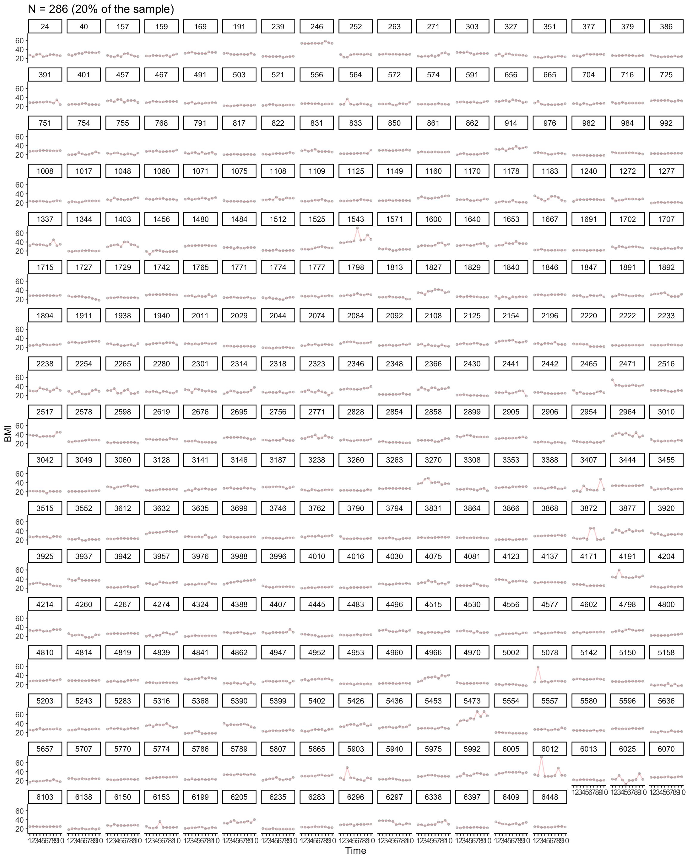
Pedro points out that waves 2016,2017,2019 have some anomolies. Here we visually inspect a subset of the data.
Show code
library(lcsm)
 # BMI
widelong <-  df %>%
  dplyr::filter(YearMeasured==1) %>%
  dplyr::filter(Wave ==2016| Wave ==2017 | Wave ==2019) %>% # k6 not measured in wave 1
  dplyr::filter(Wave!=2009) %>% # k6 not measured in wave 1
  dplyr::group_by(Id) %>% filter(n() > 2) %>%
  dplyr::select(Id, HLTH.BMI, Wave) #


wide <- spread(widelong, Wave, HLTH.BMI)

wide2 <- wide[complete.cases(wide),]
head(wide2)
# A tibble: 6 × 4
# Groups:   Id [6]
  Id    `2016` `2017` `2019`
  <fct>  <dbl>  <dbl>  <dbl>
1 2       23.2   23.2   22.9
2 15      22.8   21.4   23.1
3 16      24.7   27.4   26.2
4 19      27.0   38.3   28.9
5 20      32.2   33.3   31.6
6 21      25.9   25.9   25.1
Show code
x_var_list <- names(wide2[, 2:4])
wide2
# A tibble: 11,732 × 4
# Groups:   Id [11,732]
   Id    `2016` `2017` `2019`
   <fct>  <dbl>  <dbl>  <dbl>
 1 2       23.2   23.2   22.9
 2 15      22.8   21.4   23.1
 3 16      24.7   27.4   26.2
 4 19      27.0   38.3   28.9
 5 20      32.2   33.3   31.6
 6 21      25.9   25.9   25.1
 7 24      28.3   28.3   25.9
 8 28      33.2   35.2   35.2
 9 30      26.8   27.8   27.5
10 34      31.6   31.6   31.6
# … with 11,722 more rows
Show code
wide2 <- as.data.frame(wide2)
plot_trajectories(
  data = wide2,
  id_var = "Id",
  var_list = x_var_list,
  line_colour = "red",
  xlab = "Time",
  ylab = "BMI",
  connect_missing = F,
  scale_x_num = T,
  scale_x_num_start = 1,
  random_sample_frac = .05,
  seed = 1234
  #title_n = T
)  +
  facet_wrap( ~ Id)

BMI all
Show code
library(lcsm)
 # BMI
widelong <-  df %>%
  dplyr::filter(YearMeasured==1) %>%
 # dplyr::filter(Wave ==2016| Wave ==2017 | Wave ==2019) %>% # k6 not measured in wave 1
  dplyr::filter(Wave!=2009) %>% # k6 not measured in wave 1
  dplyr::group_by(Id) %>% filter(n() > 9) %>%
  dplyr::select(Id, HLTH.BMI, Wave) #


wide <- spread(widelong, Wave, HLTH.BMI)

wide2 <- wide[complete.cases(wide),]
head(wide2)
# A tibble: 6 × 11
# Groups:   Id [6]
  Id    `2010` `2011` `2012` `2013` `2014` `2015` `2016`
  <fct>  <dbl>  <dbl>  <dbl>  <dbl>  <dbl>  <dbl>  <dbl>
1 15      23.0   22.5   22.8   23.7   22.9   22.8   22.8
2 19      21.6   26.4   23.5   28.1   30.1   28.0   27.0
3 20      33.0   33.7   34.8   33.2   33.8   31.5   32.2
4 24      27.4   23.5   28.7   29.8   23.5   25.5   28.3
5 28      31.2   31.2   33.2   31.2   33.2   32.8   33.2
6 30      26.9   27.8   27.2   25.6   25.6   26.3   26.8
# … with 3 more variables: `2017` <dbl>, `2018` <dbl>,
#   `2019` <dbl>
Show code
x_var_list <- names(wide2[, 2:11])
wide2
# A tibble: 1,428 × 11
# Groups:   Id [1,428]
   Id    `2010` `2011` `2012` `2013` `2014` `2015` `2016`
   <fct>  <dbl>  <dbl>  <dbl>  <dbl>  <dbl>  <dbl>  <dbl>
 1 15      23.0   22.5   22.8   23.7   22.9   22.8   22.8
 2 19      21.6   26.4   23.5   28.1   30.1   28.0   27.0
 3 20      33.0   33.7   34.8   33.2   33.8   31.5   32.2
 4 24      27.4   23.5   28.7   29.8   23.5   25.5   28.3
 5 28      31.2   31.2   33.2   31.2   33.2   32.8   33.2
 6 30      26.9   27.8   27.2   25.6   25.6   26.3   26.8
 7 34      31.6   31.6   28.3   28.7   31.6   31.6   31.6
 8 38      25.8   25     25.5   26.2   25     26.2   25
 9 39      40     36.8   42.2   38.2   38.2   41.1   42.7
10 40      28.2   26.3   29.0   31.2   30.9   33.9   32.7
# … with 1,418 more rows, and 3 more variables:
#   `2017` <dbl>, `2018` <dbl>, `2019` <dbl>
Show code
wide2 <- as.data.frame(wide2)
plot_trajectories(
  data = wide2,
  id_var = "Id",
  var_list = x_var_list,
  line_colour = "red",
  xlab = "Time",
  ylab = "BMI",
  connect_missing = F,
  scale_x_num = T,
  scale_x_num_start = 1,
  random_sample_frac = .2,
  seed = 1234,
  title_n = T
)  +
  facet_wrap( ~ Id)
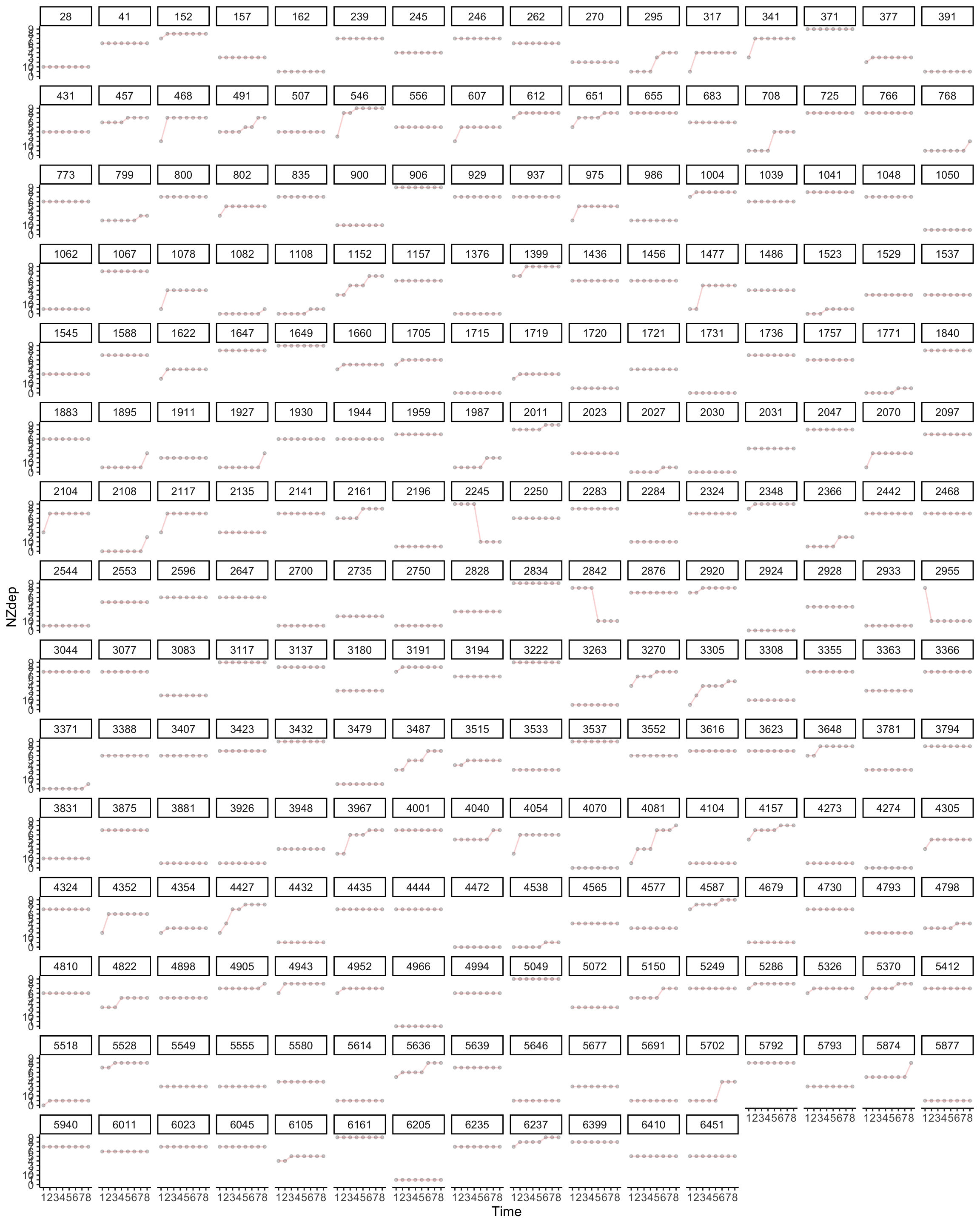
Weight
Show code
library(lcsm)
 # Weight
widelong <-  df %>%
  dplyr::filter(YearMeasured==1) %>%
  dplyr::filter(Wave ==2016| Wave ==2017 | Wave ==2019) %>% # k6 not measured in wave 1
  dplyr::filter(Wave!=2009) %>% # k6 not measured in wave 1
  dplyr::group_by(Id) %>% filter(n() > 2) %>%
  dplyr::select(Id, HLTH.Weight, Wave) #


wide <- spread(widelong, Wave, HLTH.Weight)

wide2 <- wide[complete.cases(wide),]


x_var_list <- names(wide2[, 2:4])


wide2 <- as.data.frame(wide2)
plot_trajectories(
  data = wide2,
  id_var = "Id",
  var_list = x_var_list,
  line_colour = "red",
  xlab = "Time",
  ylab = "BMI",
  connect_missing = F,
  scale_x_num = T,
  scale_x_num_start = 1,
  random_sample_frac = 0.05,
  seed = 1234
  #title_n = T
)  +
  facet_wrap( ~ Id)

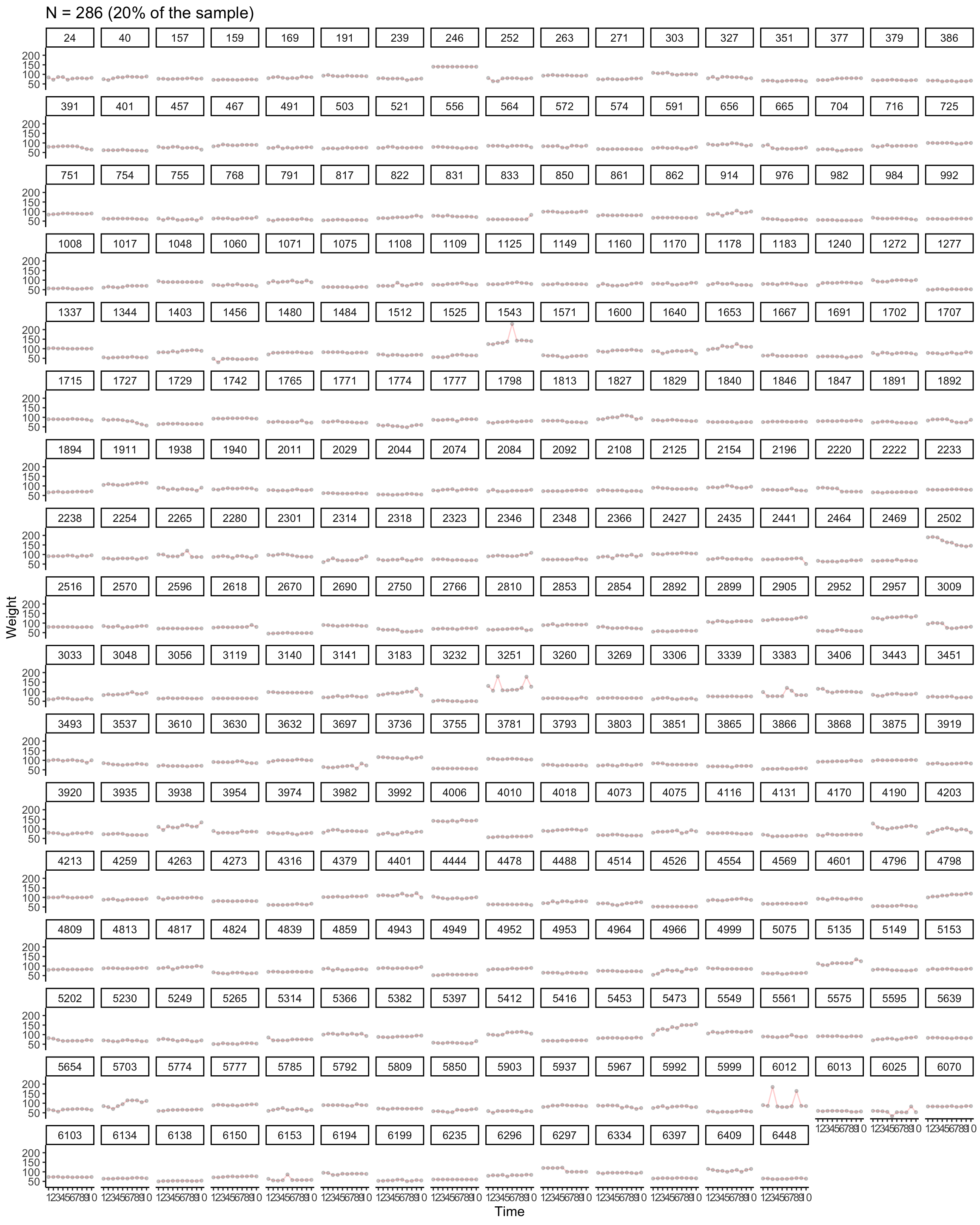
Weight all
Show code
library(lcsm)
 # Weight
widelong <-  df %>%
  dplyr::filter(YearMeasured==1) %>%
 # dplyr::filter(Wave ==2016| Wave ==2017 | Wave ==2019) %>% # k6 not measured in wave 1
  dplyr::filter(Wave!=2009) %>% # k6 not measured in wave 1
  dplyr::group_by(Id) %>% filter(n() > 9) %>%
  dplyr::select(Id, HLTH.Weight, Wave) #


wide <- spread(widelong, Wave, HLTH.Weight)
wide
# A tibble: 1,441 × 11
# Groups:   Id [1,441]
   Id    `2010` `2011` `2012` `2013` `2014` `2015` `2016`
   <fct>  <dbl>  <dbl>  <dbl>  <dbl>  <dbl>  <dbl>  <dbl>
 1 15        73     73     74     75     76     74     74
 2 19        70     72     72     72     82     81     78
 3 20        93     93     96     96     92     91     91
 4 24        84     72     86     86     72     78     80
 5 28        80     80     85     80     85     84     85
 6 30        90     90     91     83     83     89     85
 7 34        88     88     80     80     88     88     88
 8 38       103    100    102    105    100    105    100
 9 39        90     85     95     86     86     95     96
10 40        75     70     79     85     84     89     87
# … with 1,431 more rows, and 3 more variables:
#   `2017` <dbl>, `2018` <dbl>, `2019` <dbl>
Show code
wide2 <- wide[complete.cases(wide),]


x_var_list <- names(wide2[, 2:11])


wide2 <- as.data.frame(wide2)
plot_trajectories(
  data = wide2,
  id_var = "Id",
  var_list = x_var_list,
  line_colour = "red",
  xlab = "Time",
  ylab = "Weight",
  connect_missing = F,
  scale_x_num = T,
  scale_x_num_start = 1,
  random_sample_frac = 0.2,
  seed = 1234,
  title_n = T
)  +
  facet_wrap( ~ Id)
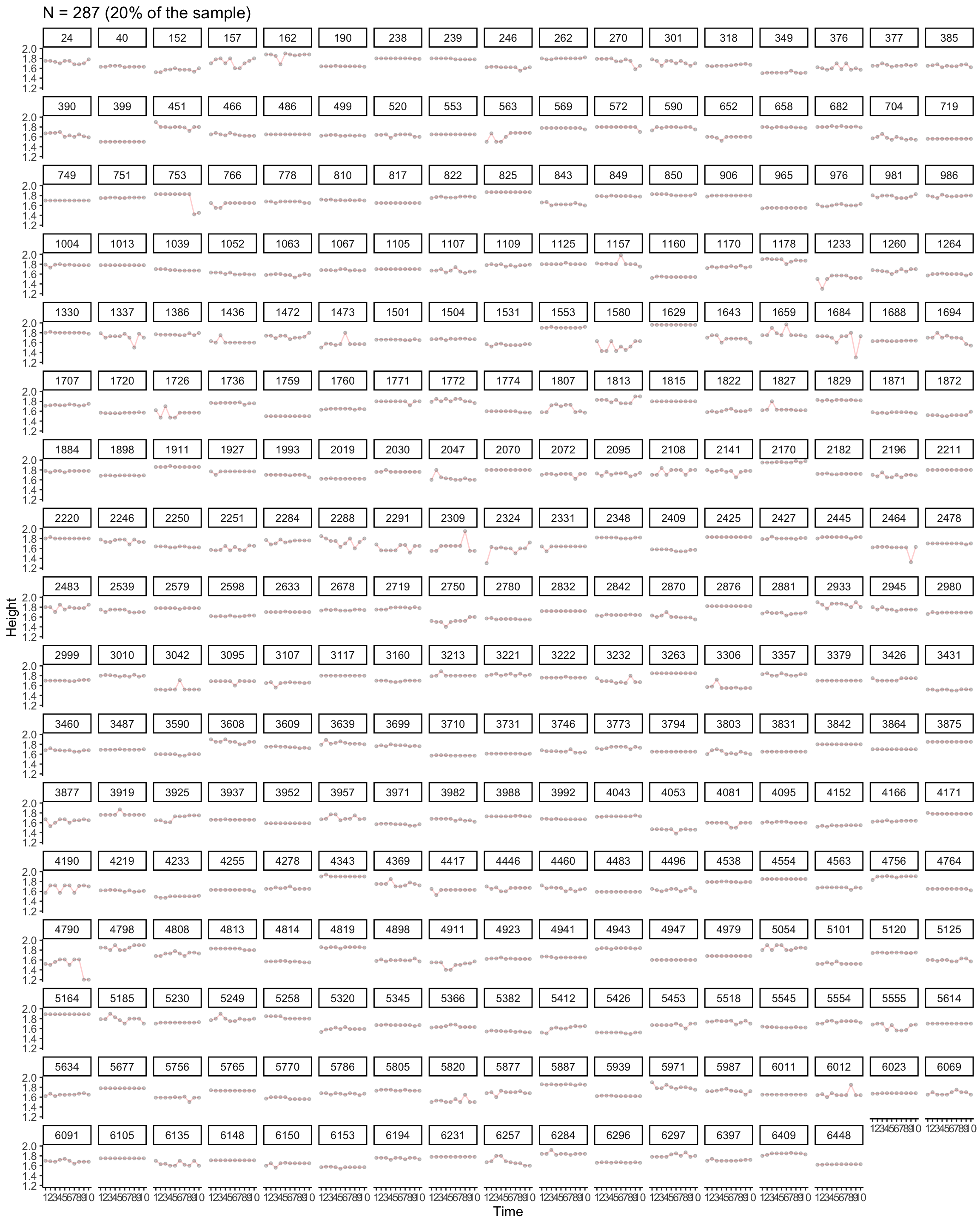
Height
Show code
library(lcsm)
 # height
widelong <-  df %>%
  dplyr::filter(YearMeasured==1) %>%
  dplyr::filter(Wave ==2016| Wave ==2017 | Wave ==2019) %>% # k6 not measured in wave 1
  dplyr::filter(Wave!=2009) %>% # k6 not measured in wave 1
  dplyr::group_by(Id) %>% filter(n() > 2) %>%
  dplyr::select(Id, HLTH.Height, Wave) #


wide <- spread(widelong, Wave, HLTH.Height)

wide2 <- wide[complete.cases(wide),]


x_var_list <- names(wide2[, 2:4])


wide2 <- as.data.frame(wide2)
plot_trajectories(
  data = wide2,
  id_var = "Id",
  var_list = x_var_list,
  line_colour = "red",
  xlab = "Time",
  ylab = "BMI",
  connect_missing = F,
  scale_x_num = T,
  scale_x_num_start = 1,
  random_sample_frac = 0.05,
  seed = 1234
  #title_n = T
)  +
  facet_wrap( ~ Id)

Height all
Show code
library(lcsm)
 # height
widelong <-  df %>%
  dplyr::filter(YearMeasured==1) %>%
#  dplyr::filter(Wave ==2016| Wave ==2017 | Wave ==2019) %>% # k6 not measured in wave 1
  dplyr::filter(Wave!=2009) %>% # k6 not measured in wave 1
  dplyr::group_by(Id) %>% filter(n() > 9) %>%
  dplyr::select(Id, HLTH.Height, Wave) #


wide <- spread(widelong, Wave, HLTH.Height)

wide2 <- wide[complete.cases(wide),]


x_var_list <- names(wide2[, 2:11])


wide2 <- as.data.frame(wide2)
plot_trajectories(
  data = wide2,
  id_var = "Id",
  var_list = x_var_list,
  line_colour = "red",
  xlab = "Time",
  ylab = "Height",
  connect_missing = F,
  scale_x_num = T,
  scale_x_num_start = 1,
  random_sample_frac = 0.2,
  seed = 1234,
  title_n = T
)  +
  facet_wrap( ~ Id)