Here we estimate the effects of the COVID-19 pandemic on Trust in Science at various stages of the pandemic in New Zealand.
Show code
# import data
df <- readRDS(here::here("data", "df"))

# prepare graph
ord_dates_class <- c(
  "Baseline",
  "JanFeb",
  "EarlyMarch",
  "Lockdown",
  "PostLockdown")

# 3665 days after 30 June 2009 Saturday 13 July 2019
# 3842 days after 30 June 2009 Monday 6 January 2020
# 3895 days after 30 June 2009 Friday 28 February 2020
# 3921 days after 30 June 2009 WED MAR 25th
# 3954 days after 30 June 2009 Monday 27 April 2020
# 3672 days after June 30 2009 Saturday 20 July 2019

# prepare data
cv <- df %>%
  dplyr::filter(YearMeasured == 1) %>%
  dplyr::filter(Wave == 2019) %>%
    droplevels() %>%
  dplyr::mutate(Covid_Timeline =
                    as.factor(ifelse(
                      TSCORE %in% 3896:3921, # feb 29 - march 25th
                      "EarlyMarch",
                      ifelse(
                        TSCORE %in% 3922:3954,
                        "Lockdown", #march 26- Mon 27 April 2020
                        ifelse(
                          TSCORE > 3954, # after april 27th 20202
                          "PostLockdown",
                          ifelse(
                            TSCORE %in% 3842:3895, # jan 6 to feb 28
                            "JanFeb",
                            "Baseline"  # 3672 TSCORE or  20 July 2019
                          )
                        )
                      )
                    ) ))%>%
  dplyr::select(
    Wave,
    TSCORE,
    SCIENCE.TRUST,
    Partner,
    Employed,
    Sat.Government,
    Id,
    Age,
    Male,
    Urban,
    Edu,
    Covid_Timeline,
    EthnicCats,
    Your.Personal.Relationships,
    Urban
  ) %>%
  dplyr::mutate(
    )%>%
  dplyr::mutate(Covid_Timeline = forcats::fct_relevel(Covid_Timeline, ord_dates_class)) %>%
  droplevels() %>%
  drop_na() %>%
  mutate(SCIENCE.TRUST_S = scale(SCIENCE.TRUST),
         Sat.Government_S = scale(Sat.Government),
         Your.Personal.Relationships_S = scale(Your.Personal.Relationships))
The New Zealand Attitudes and Values Study
- Planned 20-year longitudinal study, currently in its 12\(^{th}\) year.
- Sample frame drawn randomly from NZ Electoral Roll.
- Postal questionnaire (coverage; retention ~ 80%)
- Focus on personality, social attitudes, values, religion, meaning-making, perfectionism, virtues, habits, employment, experiences of discrimination, physical and psychological health, and environmental attitudes …
- Current sample contains
36524unique people, which is \(>\) 1% of the NZ adult population. - Here, N = 38944 longitudinal participants who responded to both 2019/20 NZAVS waves.
Table of participants per condition
Show code
| Covid_Timeline | n |
|---|---|
| Baseline | 22093 |
| JanFeb | 2540 |
| EarlyMarch | 2574 |
| Lockdown | 3189 |
| PostLockdown | 8548 |
Method
Inverse Probability Weighting
To ensure balance across the condition in baseline covariates we use Inverse Probability Weighting.
Show code
#IPW data and check weights

cobalt::bal.tab(Covid_Timeline ~  Age + Edu + EthnicCats + Male  + Urban,
        data = cv, estimand = "ATE", m.threshold = .05)
Balance summary across all treatment pairs
                      Type Max.Diff.Un      M.Threshold.Un
Age                Contin.      0.3341 Not Balanced, >0.05
Edu_0               Binary      0.0086     Balanced, <0.05
Edu_1               Binary      0.0164     Balanced, <0.05
Edu_2               Binary      0.0032     Balanced, <0.05
Edu_3               Binary      0.0144     Balanced, <0.05
Edu_4               Binary      0.0121     Balanced, <0.05
Edu_5               Binary      0.0205     Balanced, <0.05
Edu_6               Binary      0.0094     Balanced, <0.05
Edu_7               Binary      0.0070     Balanced, <0.05
Edu_8               Binary      0.0046     Balanced, <0.05
Edu_9               Binary      0.0408     Balanced, <0.05
Edu_10              Binary      0.0116     Balanced, <0.05
EthnicCats_Euro     Binary      0.0687 Not Balanced, >0.05
EthnicCats_Maori    Binary      0.0534 Not Balanced, >0.05
EthnicCats_Pacific  Binary      0.0131     Balanced, <0.05
EthnicCats_Asian    Binary      0.0179     Balanced, <0.05
Male_Male           Binary      0.0309     Balanced, <0.05
Urban_Urban         Binary      0.0218     Balanced, <0.05

Balance tally for mean differences
                    count
Balanced, <0.05        15
Not Balanced, >0.05     3

Variable with the greatest mean difference
 Variable Max.Diff.Un      M.Threshold.Un
      Age      0.3341 Not Balanced, >0.05

Sample sizes
    Baseline JanFeb EarlyMarch Lockdown PostLockdown
All    22093   2540       2574     3189         8548
Show code
# method by entropy balancing "which guarantees perfect balance on specified moments of the covariates while minimizing the entropy (a measure of dispersion) of the weights."
w_out <- WeightIt::weightit(Covid_Timeline ~ Age + Edu + EthnicCats + Male + Urban,
        data = cv, estimand = "ATE", method = "ebal")

summary(w_out)
                 Summary of weights

- Weight ranges:

                Min                                  Max
Baseline     0.8366        |-----|                1.3358
JanFeb       0.7405       |------|                1.3377
EarlyMarch   0.3499 |-------------------------|   2.2038
Lockdown     0.5122   |-------------------------| 2.3630
PostLockdown 0.6712      |--------|               1.4220

- Units with 5 greatest weights by group:

               12469   2083   5003    744   3950
     Baseline 1.2609 1.2617 1.2777 1.2924 1.3358
                6792  20019  18134  30943  14246
       JanFeb 1.3215 1.3253 1.3275 1.3333 1.3377
                3157   4943    581   3243    889
   EarlyMarch 2.0088 2.0361 2.0451 2.0799 2.2038
               16425   8141   8087  31514   5347
     Lockdown 1.9601 2.1371 2.1874 2.2753  2.363
               19492  31240   8945  33627  20012
 PostLockdown 1.3766 1.3827 1.3943 1.3953  1.422

- Weight statistics:

             Coef of Var   MAD Entropy # Zeros
Baseline           0.060 0.044   0.002       0
JanFeb             0.092 0.074   0.004       0
EarlyMarch         0.264 0.214   0.035       0
Lockdown           0.214 0.163   0.022       0
PostLockdown       0.102 0.081   0.005       0

- Effective Sample Sizes:

           Baseline  JanFeb EarlyMarch Lockdown
Unweighted 22093.   2540.      2574.    3189.
Weighted   22015.01 2518.65    2406.51  3049.22
           PostLockdown
Unweighted      8548.
Weighted        8460.07
Inspect weights:
Show code
cobalt::bal.tab(w_out, m.threshold = .05, disp.v.ratio = TRUE)
Call
 WeightIt::weightit(formula = Covid_Timeline ~ Age + Edu + EthnicCats +
    Male + Urban, data = cv, method = "ebal", estimand = "ATE")

Balance summary across all treatment pairs
                      Type Max.Diff.Adj     M.Threshold
Age                Contin.       0.0002 Balanced, <0.05
Edu_0               Binary       0.0001 Balanced, <0.05
Edu_1               Binary       0.0000 Balanced, <0.05
Edu_2               Binary       0.0001 Balanced, <0.05
Edu_3               Binary       0.0001 Balanced, <0.05
Edu_4               Binary       0.0001 Balanced, <0.05
Edu_5               Binary       0.0001 Balanced, <0.05
Edu_6               Binary       0.0000 Balanced, <0.05
Edu_7               Binary       0.0002 Balanced, <0.05
Edu_8               Binary       0.0001 Balanced, <0.05
Edu_9               Binary       0.0000 Balanced, <0.05
Edu_10              Binary       0.0001 Balanced, <0.05
EthnicCats_Euro     Binary       0.0000 Balanced, <0.05
EthnicCats_Maori    Binary       0.0000 Balanced, <0.05
EthnicCats_Pacific  Binary       0.0001 Balanced, <0.05
EthnicCats_Asian    Binary       0.0000 Balanced, <0.05
Male_Male           Binary       0.0001 Balanced, <0.05
Urban_Urban         Binary       0.0000 Balanced, <0.05
                   Max.V.Ratio.Adj
Age                         1.1722
Edu_0                            .
Edu_1                            .
Edu_2                            .
Edu_3                            .
Edu_4                            .
Edu_5                            .
Edu_6                            .
Edu_7                            .
Edu_8                            .
Edu_9                            .
Edu_10                           .
EthnicCats_Euro                  .
EthnicCats_Maori                 .
EthnicCats_Pacific               .
EthnicCats_Asian                 .
Male_Male                        .
Urban_Urban                      .

Balance tally for mean differences
                    count
Balanced, <0.05        18
Not Balanced, >0.05     0

Variable with the greatest mean difference
 Variable Max.Diff.Adj     M.Threshold
    Edu_7       0.0002 Balanced, <0.05

Effective sample sizes
           Baseline  JanFeb EarlyMarch Lockdown
Unadjusted 22093.   2540.      2574.    3189.
Adjusted   22015.01 2518.65    2406.51  3049.22
           PostLockdown
Unadjusted      8548.
Adjusted 8460.07Estimate model
Model
Show code
SCIENCE.TRUST  <- glm(
  SCIENCE.TRUST ~ Covid_Timeline,
  data = cv19w,
  weights = ipw
)
Marginal means
Show code
# estimated marginal means
means <-  estimate_means(SCIENCE.TRUST, at = "Covid_Timeline")

# print
means%>%
  print_md()
| Covid_Timeline | Mean | SE | CI_low | CI_high |
|---|---|---|---|---|
| Baseline | 5.40 | 8.50e-03 | 5.38 | 5.41 |
| JanFeb | 5.33 | 0.03 | 5.28 | 5.38 |
| EarlyMarch | 5.38 | 0.02 | 5.33 | 5.43 |
| Lockdown | 5.66 | 0.02 | 5.62 | 5.71 |
| PostLockdown | 5.57 | 0.01 | 5.54 | 5.60 |
Marginal means estimated at Covid_Timeline
Show code
#
contrasts <-  estimate_contrasts(SCIENCE.TRUST, contrast = "Covid_Timeline", adjust = "bonferroni")
contrasts%>%
  print_md()
| Level1 | Level2 | Difference | CI_low | CI_high | SE | df | t | p |
|---|---|---|---|---|---|---|---|---|
| Baseline | EarlyMarch | 0.02 | -0.05 | 0.09 | 0.03 | 38939 | 0.73 | 0.95 |
| Baseline | JanFeb | 0.07 | -7.54e-03 | 0.14 | 0.03 | 38939 | 2.52 | 0.09 |
| Baseline | Lockdown | -0.27 | -0.34 | -0.20 | 0.02 | 38939 | -11.19 | 1.33e-14 |
| Baseline | PostLockdown | -0.17 | -0.22 | -0.13 | 0.02 | 38939 | -10.73 | 4.87e-14 |
| EarlyMarch | Lockdown | -0.29 | -0.38 | -0.19 | 0.03 | 38939 | -8.57 | 4.54e-14 |
| EarlyMarch | PostLockdown | -0.19 | -0.27 | -0.11 | 0.03 | 38939 | -6.75 | 1.45e-10 |
| JanFeb | EarlyMarch | -0.05 | -0.15 | 0.05 | 0.04 | 38939 | -1.35 | 0.66 |
| JanFeb | Lockdown | -0.33 | -0.43 | -0.24 | 0.03 | 38939 | -9.96 | 4.20e-14 |
| JanFeb | PostLockdown | -0.24 | -0.32 | -0.16 | 0.03 | 38939 | -8.39 | 5.16e-14 |
| Lockdown | PostLockdown | 0.10 | 0.02 | 0.17 | 0.03 | 38939 | 3.62 | 2.68e-03 |
Marginal contrasts estimated at Covid_Timeline p-value adjustment method: Bonferroni
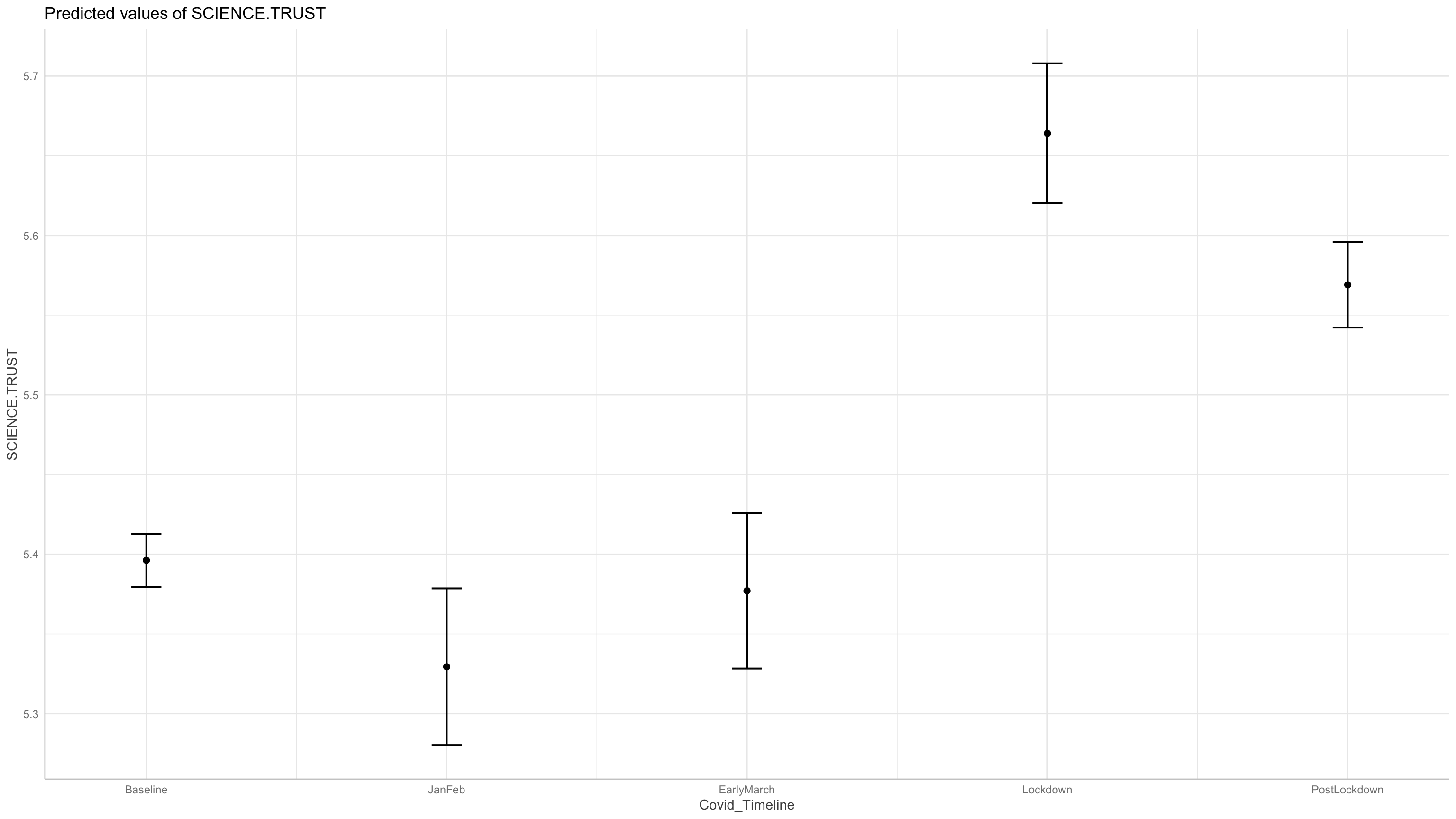
Graph of the expected (marginal) means:
Show code
#plot(means, alpha =.005)
ggplot(cv19w, aes(x = Covid_Timeline, y = SCIENCE.TRUST)) +
  # Add base data
  geom_violin(aes(fill = Covid_Timeline), color = "white") +
  geom_jitter2(width = 0.05, alpha = 0.005) +
  # Add pointrange and line from means
  geom_line(data = means, aes(y = Mean, group = 1), size = .3) +
  geom_pointrange(
    data = means,
    aes(y = Mean, ymin = CI_low, ymax = CI_high),
    size = .3,
    color = "white"
  ) +
  # Improve colors
  scale_fill_material() +
  theme_modern() +
  scale_color_discrete()
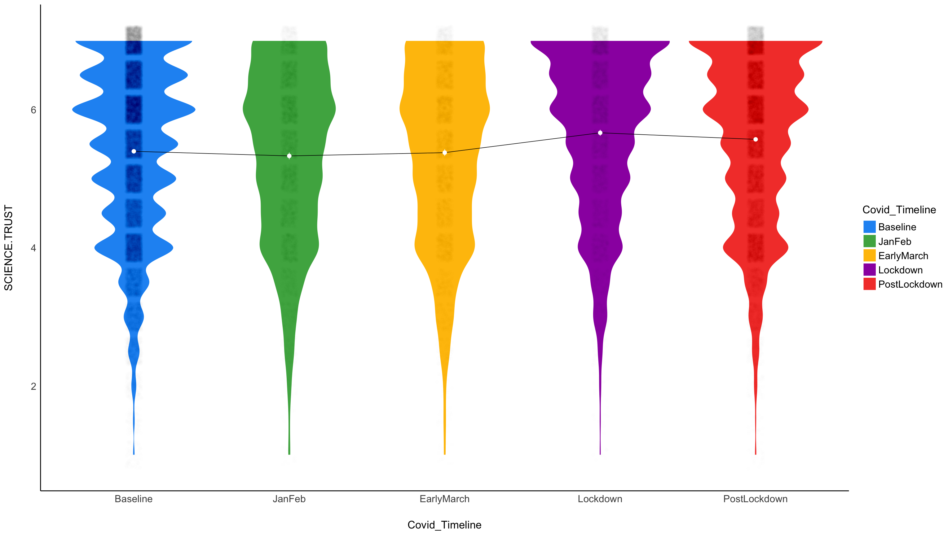
Trust in science increased, and then dropped. The key question, will it trust revert to baseline (or worse)?
Below another graph of the same result.
Causal mediation model
Show code
library(mediation)
#length(unique(cv19n$Id))

# + Age + Edu + EthnicCats + Male + Relid + Partner + Urban

med.fit <- lm( Sat.Government_S  ~ Covid_Timeline + Age + Edu + EthnicCats + Male  + Urban,  data = cv19w)
out.fit <- lm( SCIENCE.TRUST_S   ~ Sat.Government_S  + Covid_Timeline +  Age + Edu + EthnicCats + Male + Urban,
               data = cv19w)
med.out <- mediate(med.fit, out.fit, treat = "Covid_Timeline", mediator = "Sat.Government_S",
                   robustSE = TRUE, sims = 1000, control.value = "Baseline", treat.value = "Lockdown")

# save model
saveRDS(med.out, here::here("_posts", "covscience","mods", "med.out.rds"))
We observe that government satisfaction strongly mediates the effect of Lockdown on trust in science.
Show code
Causal Mediation Analysis

Quasi-Bayesian Confidence Intervals

               Estimate 95% CI Lower 95% CI Upper p-value
ACME             0.1041       0.0951         0.11  <2e-16
ADE              0.1078       0.0726         0.14  <2e-16
Total Effect     0.2119       0.1775         0.25  <2e-16
Prop. Mediated   0.4923       0.4184         0.60  <2e-16

ACME           ***
ADE            ***
Total Effect   ***
Prop. Mediated ***
---
Signif. codes:
0 '***' 0.001 '**' 0.01 '*' 0.05 '.' 0.1 ' ' 1

Sample Size Used: 38944


Simulations: 1000 
We next contrast the Locdown with the period following lockdown in which there was declining trust in science.
Sensitivity Analysis
Sensitivity plot reveals that for sequential ignorability to be violated, the correlation between the the error terms of the mediator and outcome (rho) would need to be .25. We infer that the findings are reasonably robust in respect of unmeasured mediator outcome confounding.
Show code
sens.out <- readRDS(sens.out, here::here("_posts", "covscience","mods", "sens.out.rds"))

#summary(sens.out)
plot(sens.out)
#plot(sens.out, sens.par = "R2", r.type = "total", sign.prod = "positive")
# This is the workhorse function for sensitivity analyses for average causal mediation effects. The sensitivity analysis can be used to assess the robustness of the findings from mediate to the violation of sequential ignorability, the crucial identification assumption necessary for the estimates to be valid. The analysis proceeds by quantifying the degree of sequential ignorability violation as the correlation between the error terms of the mediator and outcome models, and then calculating the true values of the average causal mediation effect for given values of this sensitivity parameter, rho. The original findings are deemed sensitive if the true effects are found to vary widely as function of rho.

#The resulting "rho" figures plot the estimated true values of ACME (or ADE, proportion mediated) against rho, along with the confidence intervals. When rho is zero, sequantial ignorability holds, so the estimated value at that point will be equal to the estimate returned by the mediate. The confidence level is determined by the 'conf.level' value of the original mediate object
Negative Controls
Show code
med.fitR <- lm( Your.Personal.Relationships_S  ~ Covid_Timeline + Age + Edu + EthnicCats + Male  + Urban,  data = cv19w)
out.fitR <- lm( SCIENCE.TRUST_S   ~ Your.Personal.Relationships_S  + Covid_Timeline +  Age + Edu + EthnicCats + Male + Urban,
               data = cv19w)
med.outR <- mediate(med.fitR, out.fitR, treat = "Covid_Timeline", mediator = "Your.Personal.Relationships_S",
                   robustSE = TRUE, sims = 1000, control.value = "Baseline", treat.value = "Lockdown")

# save model
saveRDS(med.outR, here::here("_posts", "covscience","mods", "med.outR.rds"))
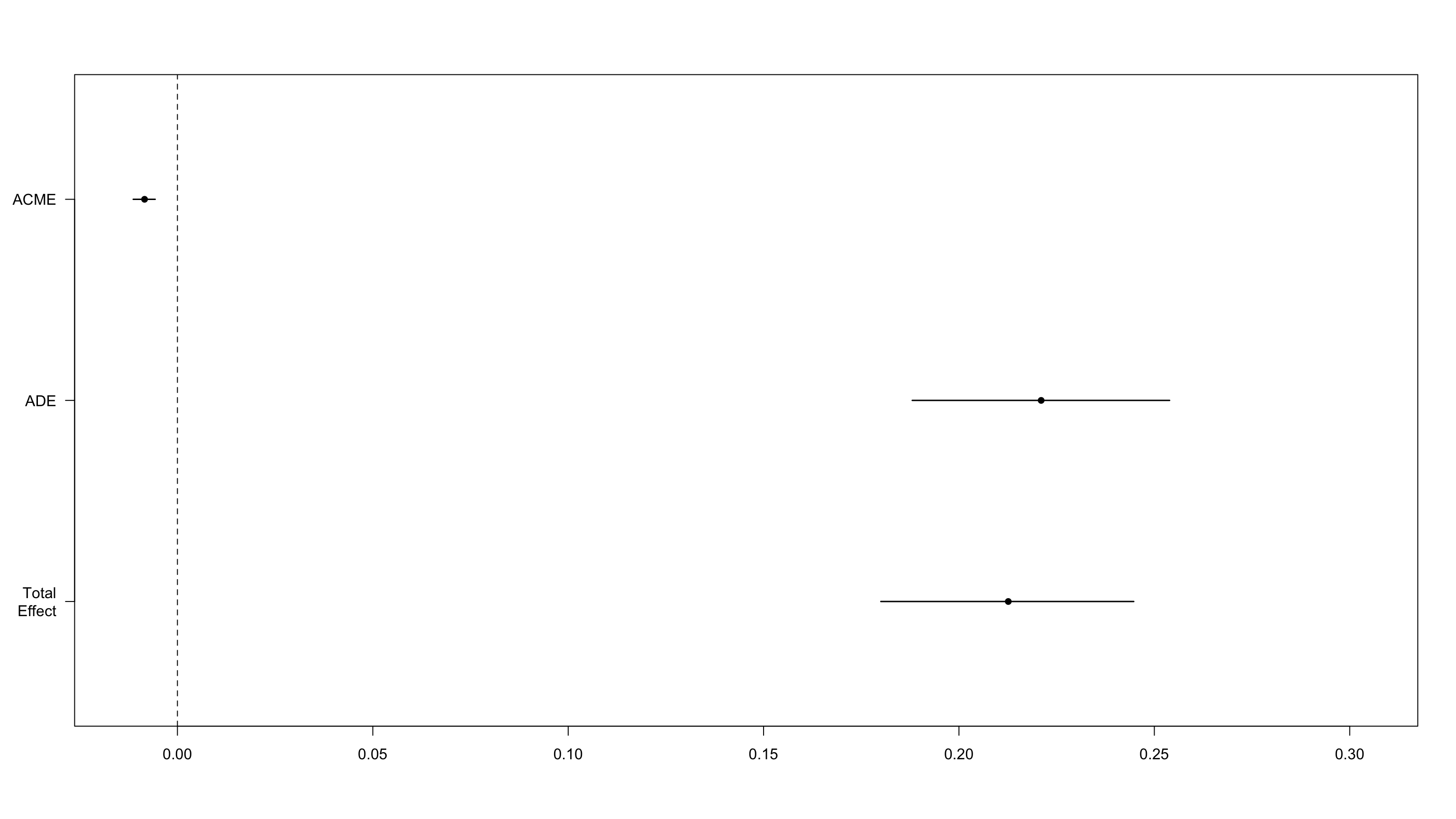
We do not find an effect for satisfaction with relationships
Show code
Causal Mediation Analysis

Quasi-Bayesian Confidence Intervals

               Estimate 95% CI Lower 95% CI Upper p-value
ACME           -0.00841     -0.01132        -0.01  <2e-16
ADE             0.22104      0.18804         0.25  <2e-16
Total Effect    0.21262      0.18001         0.24  <2e-16
Prop. Mediated -0.03920     -0.05643        -0.03  <2e-16

ACME           ***
ADE            ***
Total Effect   ***
Prop. Mediated ***
---
Signif. codes:
0 '***' 0.001 '**' 0.01 '*' 0.05 '.' 0.1 ' ' 1

Sample Size Used: 38944


Simulations: 1000
Show code
plot(med.outR)
Reverse causation
We next investigate whether declining satisfaction with government caused a drop in trust in science (reverse causal model)
We find evidence for only a weak mediation effect
Show code
Causal Mediation Analysis

Quasi-Bayesian Confidence Intervals

               Estimate 95% CI Lower 95% CI Upper p-value
ACME            -0.0222      -0.0288        -0.02  <2e-16
ADE             -0.0542      -0.0881        -0.02  <2e-16
Total Effect    -0.0765      -0.1104        -0.04  <2e-16
Prop. Mediated   0.2863       0.1853         0.60  <2e-16

ACME           ***
ADE            ***
Total Effect   ***
Prop. Mediated ***
---
Signif. codes:
0 '***' 0.001 '**' 0.01 '*' 0.05 '.' 0.1 ' ' 1

Sample Size Used: 39746


Simulations: 1000
Show code
plot(med.out2)
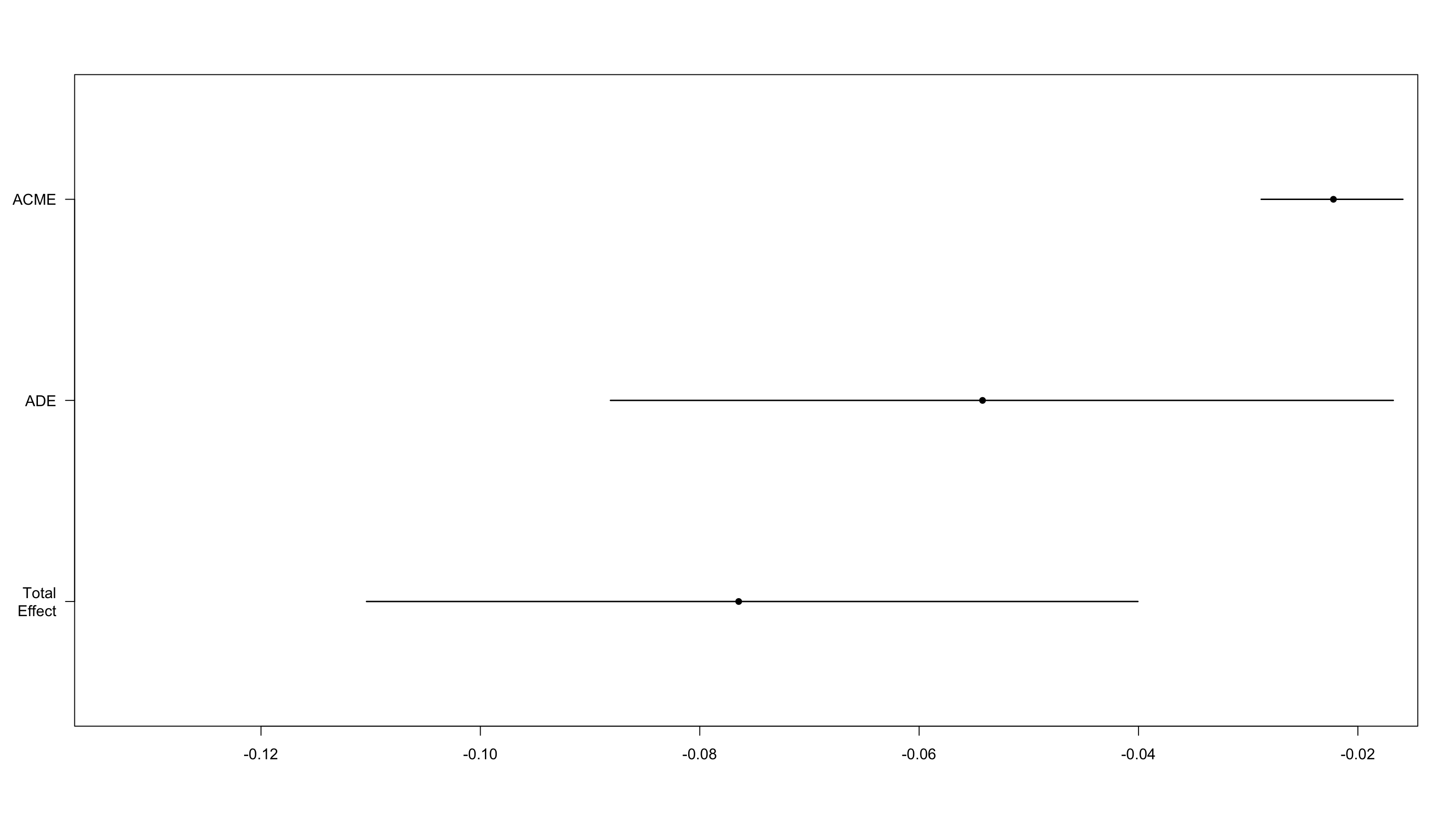
As expected this small effect is robust to unmeasured confounding.
Does trust in science mediate the effect of government satisfaction?
Show code
med.fitb <- lm( SCIENCE.TRUST_S  ~ Covid_Timeline + Age + Edu + EthnicCats + Male  + Urban,  data = cv19w)
out.fitb <- lm( Sat.Government_S   ~ SCIENCE.TRUST_S  + Covid_Timeline +  Age + Edu + EthnicCats + Male + Urban,
               data = cv19w)
med.outb <- mediate(med.fitb, out.fitb, treat = "Covid_Timeline", mediator = "SCIENCE.TRUST_S",
                   robustSE = TRUE, sims = 1000, control.value = "Baseline", treat.value = "Lockdown")

saveRDS(med.outb, here::here("_posts", "covscience","mods", "med.outb.rds"))
We find a very strong effect of lockdown on satisfaction with government, but we do not find any evidence for a substantial effect of mediation through trust in science.
Show code
Causal Mediation Analysis

Quasi-Bayesian Confidence Intervals

               Estimate 95% CI Lower 95% CI Upper p-value
ACME             0.0362       0.0299         0.04  <2e-16
ADE              0.5815       0.5472         0.62  <2e-16
Total Effect     0.6177       0.5850         0.65  <2e-16
Prop. Mediated   0.0584       0.0485         0.07  <2e-16

ACME           ***
ADE            ***
Total Effect   ***
Prop. Mediated ***
---
Signif. codes:
0 '***' 0.001 '**' 0.01 '*' 0.05 '.' 0.1 ' ' 1

Sample Size Used: 39746


Simulations: 1000 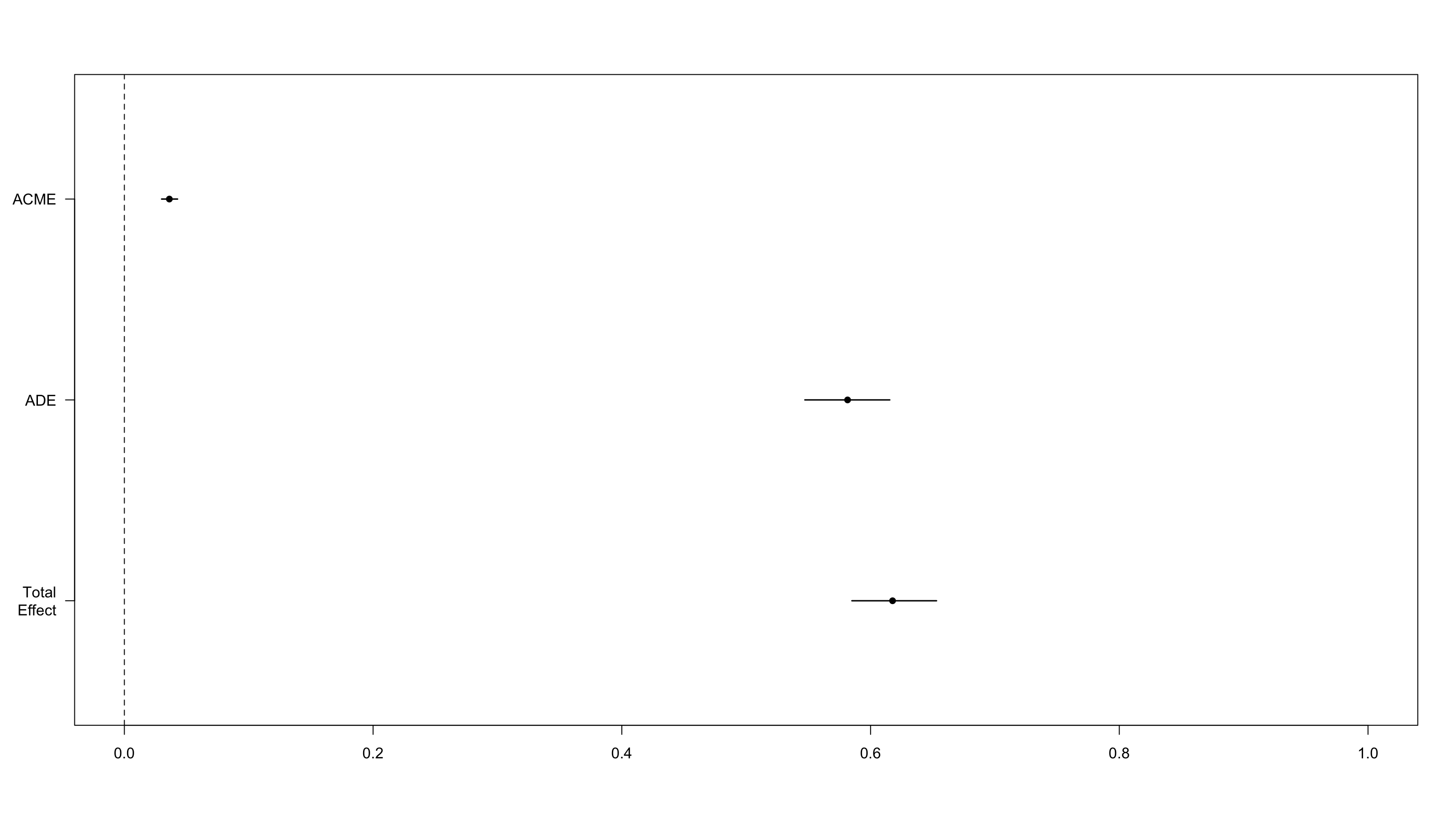
Sensitivity analysis
Show code
sens.outb2 <- medsens(med.outb2, rho.by = 0.25,  effect.type = "indirect", sims = 100)
# save sensitivity analysis
saveRDS(sens.outb2, here::here("_posts", "covscience","mods", "sens.outb2.rds"))
sens.outb2 <- readRDS(here::here("_posts", "covscience","mods", "sens.outb2.rds"))
plot(sens.outb2)
summary(sens.outb2)
Loss of gov’t satisfaction does not mediate loss of trust in science.
We can ask whether the fall in government satisfaction was mediated by a loss of confidence in science.
We do not find strong evidence for a causal effect of loss of trust in science on satisfaction with the government.
Show code
Causal Mediation Analysis

Quasi-Bayesian Confidence Intervals

               Estimate 95% CI Lower 95% CI Upper p-value
ACME            -0.0130      -0.0194        -0.01  <2e-16
ADE             -0.1197      -0.1575        -0.08  <2e-16
Total Effect    -0.1326      -0.1715        -0.09  <2e-16
Prop. Mediated   0.0973       0.0497         0.16  <2e-16

ACME           ***
ADE            ***
Total Effect   ***
Prop. Mediated ***
---
Signif. codes:
0 '***' 0.001 '**' 0.01 '*' 0.05 '.' 0.1 ' ' 1

Sample Size Used: 39746


Simulations: 1000
Show code
# covid timeline
# 3665 days after 30 June 2009 Saturday 13 July 2019
# 3842 days after 30 June 2009 Monday 6 January 2020
# 3895 days after 30 June 2009 Friday 28 February 2020
# 3921 days after 30 June 2009 WED MAR 25th
library(lubridate)
library(tidyverse)

carep <- cv %>%
  dplyr::mutate(timeline = make_date(year = 2009, month = 6, day = 30) + TSCORE) %>%
  count(day = floor_date(timeline, "day")) %>%
dplyr::mutate(condition = ifelse(
  #    day >= "2019-06-20" &
        day < "2020-01-06",
      "Baseline",
      ifelse(
        day >= "2020-01-06" & day < "2020-02-29",
        "JanFeb",
        ifelse(
          day >= "2020-02-29" & day < "2020-03-25",
          "EarlyMarch",
          ifelse(
            day >= "2020-03-25" &
              day < "2020-04-28",
            "Lockdown",
            "PostLockdown"
            ))))) %>%
  dplyr::mutate(condition = forcats::fct_relevel(condition, ord_dates_class)) %>%
  arrange(day)


# get COVID date
minday <- min(carep$day) # min day
dates_vline1<- as.Date(minday) # min day
dates_vline2<- as.Date("2020-01-06")
dates_vline3<- as.Date("2020-02-28")
# get data of change of baseline
dates_vline4<- as.Date("2020-03-25")
dates_vline5 <- as.Date("2020-04-27")
dates_vline6 <- as.Date("2020-10-15") # end day
# for line in a graph

# for line in a graph
#
dates_vline1b <- which(carep$day %in% dates_vline1)
dates_vline2b <- which(carep$day %in% dates_vline2)
dates_vline3b <- which(carep$day %in% dates_vline3)
dates_vline4b <- which(carep$day %in% dates_vline4)
dates_vline5b <- which(carep$day %in% dates_vline5)
dates_vline6b <- which(carep$day %in% dates_vline6)


tline <- ggplot(carep, aes(day, n)) +
  geom_col(aes(fill = condition)) + scale_x_date(date_labels = "%b/%Y", limits = c(as.Date(minday),
                                                                                   as.Date("2020-10-15")))  +
  scale_y_continuous(limits = c(0, 1000))  +
  geom_vline(xintercept = as.numeric(carep$day[dates_vline1b]),
             col = "red",
             linetype = "dashed") +
  geom_vline(xintercept = as.numeric(carep$day[dates_vline2b]),
             col = "red") +
  geom_vline(xintercept = as.numeric(carep$day[dates_vline3b]),
             col = "red",
             linetype = "dashed") +
  geom_vline(xintercept = as.numeric(carep$day[dates_vline4b]),
             col = "red",
             linetype = "dashed") +
  geom_vline(xintercept = as.numeric(carep$day[dates_vline5b]),
             col = "red",
             linetype = "dashed") +
  xlab("NZAVS Waves 10 and 11 daily counts: repeated measures") + ylab("Count of Responses")  + theme_classic() +   scale_fill_viridis_d() + theme(
    legend.position = "top",
    legend.text = element_text(size = 6),
    legend.title = element_text(color = "Black", size = 8)) +
  # annotate(
  #   "rect",
  #   xmin = as.Date("2019-06-20"),
  #   xmax = dates_vline1,
  #   ymin = 0,
  #   ymax = 1000,
  #   alpha = .1,
  #   fill = "darkblue"
  # )  +
  # annotate(
  #   "rect",
  #   xmin = dates_vline1,
  #   xmax = dates_vline6,
  #   ymin = 0,
  #   ymax = 1000,
  #   alpha = .001
  # ) +
  # annotate(
  #   geom = "curve",
  #   x = as.Date("2019-06-20"),
  #   y = 750,
  #   xend = as.Date("2019-10-15"),
  #   yend = 800,
  #   curvature = -.2,
  #   arrow = arrow(length = unit(2, "mm"))
  # ) +
  # annotate(
  #   geom = "curve",
  #   x = as.Date("2019-06-20"),
  #   y = 750,
  #   xend = as.Date("2020-01-30"),
  #   yend = 850,
  #   curvature = -.2,
  #   arrow = arrow(length = unit(2, "mm"))
  # ) +
  # annotate(
  #   geom = "curve",
  #   x = as.Date("2019-06-20"),
  #   y = 750,
  #   xend = as.Date("2020-03-10"),
  #   yend = 875,
  #   curvature = -.2,
  #   arrow = arrow(length = unit(2, "mm"))
  # ) +
  # annotate(
  #   geom = "curve",
  #   x = as.Date("2019-06-20"),
  #   y = 750,
  #   xend = as.Date("2020-04-10"),
  #   yend = 900,
  #   curvature = -.2,
  #   arrow = arrow(length = unit(2, "mm"))
  # ) +
  # annotate(
  #   geom = "curve",
  #   x = as.Date("2019-06-20"),
  #   y = 750,
  #   xend = as.Date("2020-06-10"),
  #   yend = 925,
  #   curvature = -.2,
  #   arrow = arrow(length = unit(2, "mm"))
  # ) +
  annotate("text",
           x = as.Date("2019-06-20"),
           y = 755,
           label = "0") +
  annotate("text",
           x = as.Date("2019-10-25"),
           y = 800,
           label = "1") +
   annotate("text",
           x = as.Date("2020-02-10"),
           y = 850,
           label = "2") +
  annotate("text",
           x = as.Date("2020-03-15"),
           y = 875,
           label = "3") +
  annotate("text",
           x = as.Date("2020-04-20"),
           y = 900,
           label = "4") +
  annotate("text",
           x = as.Date("2020-06-10"),
           y = 925,
           label = "5")
Appendix
Graph of timeline
Show code
# GRAPH
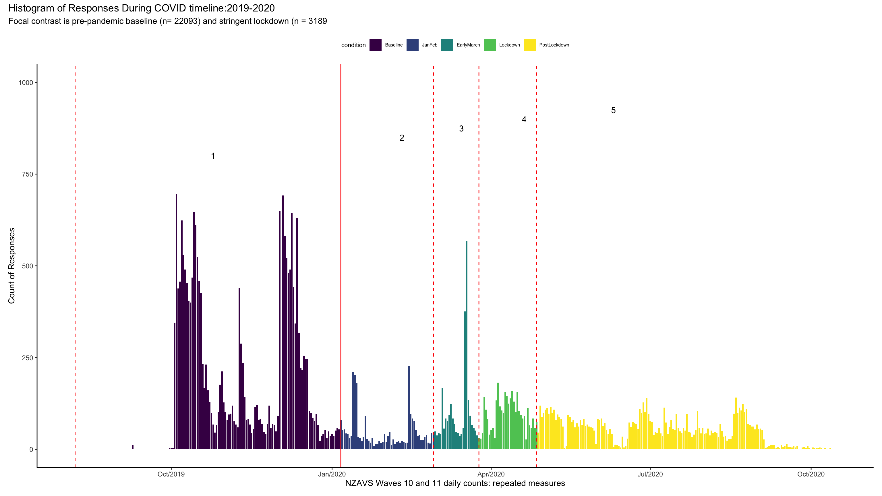
tline + plot_annotation(title = "Histogram of Responses During COVID timeline:2019-2020",
subtitle = "Focal contrast is pre-pandemic baseline (n= 22093) and stringent lockdown (n = 3189")