M-Bias: Confounding Control Using Three Waves of Panel Data

Review

Elsewhere, we have described our strategy for using three waves of panel data to identify causal effects. For confounding control, we adopt VanderWeele’s modified disjunctive cause criterion:

control for each covariate that is a cause of the exposure, or of the outcome, or of both; exclude from this set any variable known to be an instrumental variable; and include as a covariate any proxy for an unmeasured variable that is a common cause of both the exposure and the outcome (VanderWeele, Mathur, and Chen 2020, 441; VanderWeele 2019).

Such a criterion might appear to be too liberal. It might seem that we should instead select the minimum adjustment set of confounders necessary for confounding control. Of course, the minimum adjustment set cannot generally be known. However, a liberal inclusion criterion would seem to invite confounding by over-conditioning. We next consider the risks of such liberality in three-wave panel designs.

M-bias

M-bias is a form of bias that can arise when we include too many variables in our analysis, a phenomenon known as over-conditioning. Let’s break this down using a concrete example.

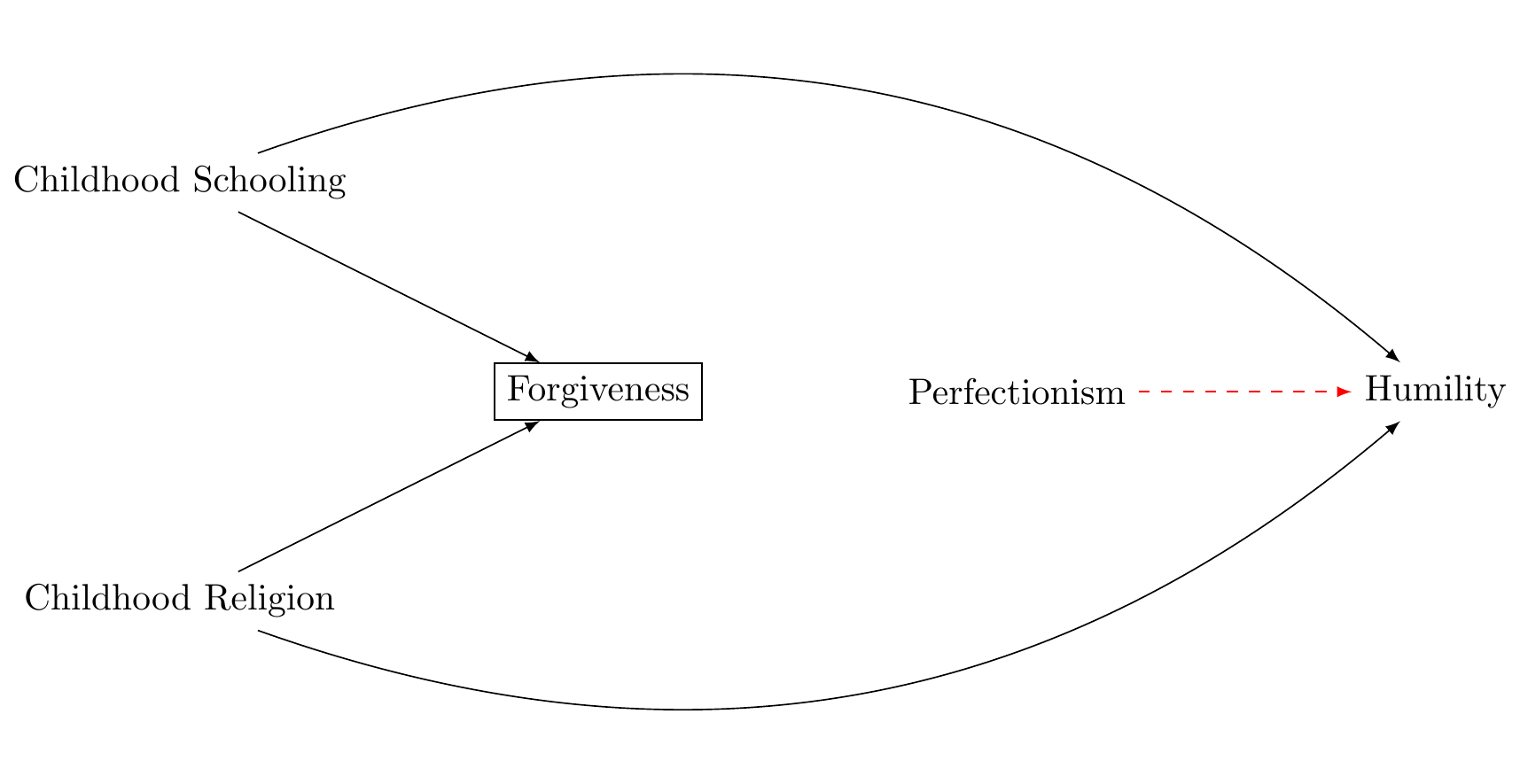
Suppose we’re interested in understanding if being a perfectionist influences a person’s level of humility. We start with the assumption that there’s no direct cause-and-effect relationship between perfectionism (the exposure) and humility (the outcome).

Now imagine we’re including forgiveness in our analysis. We know that childhood schooling influences both forgiveness and perfectionism, and childhood religion affects forgiveness and humility. If we adjust for forgiveness in our analysis, an indirect path (or backdoor path) is created between perfectionism and humility, leading to M-bias. This path can be illustrated as Figure 1.

Figure 1: M-bias: an example of confounding that arises from over-adjustment

By including forgiveness in our model, we’ve inadvertently introduced a correlation between perfectionism and humility where one didn’t previously exist. This is the essence of M-bias.

The Power of Baseline Measures

One might think the solution is simple - don’t include forgiveness in the model. However, our understanding of causal relationships is often imperfect, and there may be plausible reasons to believe that forgiveness does, in fact, influence perfectionism. If this were the case, to avoid bias, we would need to condition on a proxy of the unmeasured variables. This strategy might not completely avoid bias, which is why it is important to include sensitivity analyses to assess how much unmeasured confounding would be required to explain a result away (VanderWeele and Ding 2017)

Conclusion

In our pursuit of understanding causal relationships, we must carefully navigate the risk of M-bias—a form of confounding that can emerge from over-adjusting for variables. We’ve outlined a strategy to mitigate this bias by including both prior measurements of the exposure and the outcome in our studies. This approach provides a robust mechanism to control for unmeasured confounders that might otherwise skew our results. However, even with these measures, we cannot guarantee the elimination of all confounding. For this reason, we also conduct sensitivity analysis using E-values to assess the robustness of our findings to potential unmeasured confounding. E-values provide a quantitative measure of the minimum strength an unmeasured confounder would need to fully explain away an observed association.

In future posts, we will delve more deeply into the concept of E-values and their role in robust causal inference. By leveraging strategies for confounding control that include previous measures of the outcome and exposure variables, as well as senstivity analysis, we strive for more reliable, accurate insights in our studies.

Acknowledgements

I am grateful to Templeton Religion Trust Grant 0418 for supporting my work.¹

References

VanderWeele, Tyler J. 2019. “Principles of Confounder Selection.” European Journal of Epidemiology 34 (3): 211219.

VanderWeele, Tyler J, and Peng Ding. 2017. “Sensitivity Analysis in Observational Research: Introducing the e-Value.” Annals of Internal Medicine 167 (4): 268274.

VanderWeele, Tyler J, Maya B Mathur, and Ying Chen. 2020. “Outcome-Wide Longitudinal Designs for Causal Inference: A New Template for Empirical Studies.” Statistical Science 35 (3): 437466.

Footnotes

1. The funders played no role in the design or interpretation of this research.