What is Inverse Probability of Treatment Weighting (IPTW)?
Inverse Probability of Treatment Weighting (IPTW) is a method for estimating causal effects from observational data, using propensity scores to balance covariates between treated and untreated groups. This creates a pseudo-population where the probability of treatment assignment is independent of the observed covariates (gender, in our example below). Similar to G-computation, the method helps to estimate causal effects more accurately.
Here, we consider IPTW in a setting where we wish to estimate the Average Treatment Effect (ATE).
Bias in observational data: an example
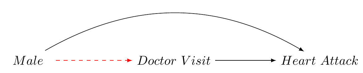
Consider an observational dataset with measures for gender (L), frequency of doctor’s visits (our treatment A), and heart attack incidence (our outcome Y).
Let’s assume:
- The 10-year incidence risk of heart attacks is \(p\) for females.
- For males, the risk is \(2p\) (twice as high).
- Doctor visits reduce the risk of heart attacks by \(0.2p\).
- Males are half as likely to visit doctors as females.
In our sample of 1,000 individuals:
- 500 are males (50% of 1,000)
- 500 are females (50% of 1,000)
The overall risk \(R_{\text{sample}}\) in the sample is computed as the weighted sum of the risks in males and females:
\(R_{\text{sample}} = 0.5 \times 2p + 0.5 \times p = 1.5p\)
Given that the gender proportions are balanced in our sample, \(R_{\text{sample}}\) should also represent the true risk \(R_{\text{population}}\) in the population:
\(R_{\text{population}} = R_{\text{sample}} = 1.5p\)
However, if we also suppose:
- Doctor’s visits (the treatment) reduce the risk of a heart attack by \(0.25p\).
- Males are twice less likely to visit doctors than females.
Under these conditions, the causal effect of treatment on the outcome will be biased.
We assume the baseline risk for females is \(0.2\) and for males is \(0.4\) (since they are twice as likely to have heart attacks). The treatment effect for individuals who visit a doctor (both males and females) reduces their risk by \(0.25p\).
Hence, we have:
- Risk of heart attack for females who do not visit the doctor: \(0.2\)
- Risk of heart attack for females who visit the doctor: \(0.2 - 0.25 \times 0.2 = 0.15\)
- Risk of heart attack for males who do not visit the doctor: \(0.4\)
- Risk of heart attack for males who visit the doctor: \(0.4 - 0.25 \times 0.4 = 0.3\)
The bias in the sample is represented in the causal graph Figure 1.
We represent the treatment group (doctor’s visits) and control group (no doctor’s visits) as A = 1 and A = 0, respectively, and simulate our data:
| Actual_Treatment | A_1 | A_0 |
|---|---|---|
| Male | .25 | .75 |
| Female | .75 | .25 |
Code
library(tidyverse)
library(knitr)
library(kableExtra)

# create data frame
my_data <- tibble(
 Weighted_Treatment = c(
 "Male",
 "Female"),
 A_1 = c(".5", ".5"),
 A_0 = c(".5", ".5"),
)

# create table
my_data %>%
 kbl(format = "html") |>
kable_styling("hover")| Weighted_Treatment | A_1 | A_0 |
|---|---|---|
| Male | .5 | .5 |
| Female | .5 | .5 |
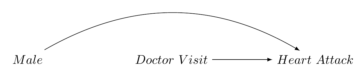
Addressing bias using IPTW
Mathematically, the ATE using IPTW can be represented as follows: ### Inverse Probability of Treatment Weighting (IPTW) Estimator
Step 1 Estimate the propensity score. The propensity score \(\hat{e}\) is the conditional probability of the exposure \(A = 1\), given the covariates \(L\). This can be modelled using logistic regression or other suitable methods, depending on the nature of the data and the exposure.
\[e = P(A = 1 | L) = f_A(L; \theta_A)\]
Here, \(f_A(L; \theta_A)\) is a function that estimates the probability of the exposure \(A = 1\) given covariates \(L\). (In classical IPTW, the model is a logistic or multinomial model for the treatment, predicted by covariates that are also associated with the outcome.) Then, we calculate the weights for each individual, denoted as \(v\), using the estimated propensity score:
\[ v = \begin{cases} \frac{1}{e} & \text{if } A = 1 \\ \frac{1}{1-e} & \text{if } A = 0 \end{cases} \]
Thus, \(v\) depends on \(A\), and is calculated as the inverse of the propensity score for exposed individuals and as the inverse of \(1-e\) for unexposed individuals.
Step 2 Fit a weighted outcome model. Using the weights calculated from the estimated propensity scores, fit a model for the outcome \(Y\), conditional on the exposure \(A\). This can be represented as:
\[ \hat{E}(Y|A; V) = f_Y(A ; \theta_Y, V) \]
In this model, \(f_Y\) is a function (here, a weighted regression model) with parameters \(θ_Y\). The weights \(V\) are incorporated into the estimation process, affecting how much each observation contributes to the estimation of \(θ_Y\), but they are not themselves an additional variable within the model.
Step 3 Simulate potential outcomes. For each individual, simulate their potential outcome under the hypothetical scenario where everyone is exposed to the intervention \(A=a\) regardless of their actual exposure level:
\[\hat{E}(a) = \hat{E}[Y_i|A=a; \hat{\theta}_Y, v_i]\]
and also under the hypothetical scenario where everyone is exposed to intervention \(A=a'\):
\[\hat{E}(a') = \hat{E}[Y_i|A=a'; \hat{\theta}_Y, v_i]\]
Thus the expectation is calculated for each individual \(i\), with individual-specific weights \(v_i\).
Step 4 Estimate the average causal effect as the difference in the predicted outcomes:
\[\hat{\delta} = \hat{E}[Y(a)] - \hat{E}[Y(a')]\]
The estimated difference \(\hat{\delta}\) represents the average causal effect. (In NZAVS research we use simulation-based inference methods to compute standard errors and confidence intervals using the clarify` package in R (Greifer et al. 2023) (Note, in the following illustration, for simplicity, we use monte-carlo simulation)
Simulation
# Load necessary libraries
library(tidyverse)

# Note
#1. **Treatment assignment:** Treatment assignment must be randomized within each gender group.

#2. **Outcome calculation:** In the calculation of the outcome,the treatment effect should only apply to those who received the treatment.

#3. **IPTW weight calculation:** The weights are  the inverse probability of treatment weights (IPTW), which are used to create a pseudo-population in which treatment assignment is independent of the observed covariates.

#4. **ATE calculation:** The ATE should be calculated as the difference in the mean outcomes between the treated and untreated groups in the IPTW-adjusted population.


# Function to generate data and calculate ATE
simulate_ATE <- function() {
  # Define groups
  N <- 1000

  # Define the risks
  risk_F <- 0.4
  risk_M <- 0.6
  risk_reduction <- 0.25

  # Create a data frame
  data <- tibble(
    gender = rep(c("Female", "Male"), each = N/2),
    treatment = c(rbinom(N/2, 1, 0.6), rbinom(N/2, 1, 0.2))  # Treatment assignment based on propensity scores
  )

  # Define outcome based on gender, treatment, and associated risk
  data <- data %>%
    mutate(outcome = ifelse(gender == "Female",
                            ifelse(treatment == 1, rbinom(N/2, 1, risk_F - risk_reduction), rbinom(N/2, 1, risk_F)),
                            ifelse(treatment == 1, rbinom(N/2, 1, risk_M - risk_reduction), rbinom(N/2, 1, risk_M))))

  # Generate propensity scores using logistic regression
  model_ps <- glm(treatment ~ gender, data = data, family = "binomial")
  data$ps <- predict(model_ps, type = "response")

  # Calculate IPTW weights
  data <- data %>% mutate(weight = ifelse(treatment == 1, 1/ps, 1/(1-ps)))

  # Calculate ATE using IPTW
  treated_outcome <- with(data, sum(weight[outcome == 1 & treatment == 1]) / sum(weight[treatment == 1]))
  control_outcome <- with(data, sum(weight[outcome == 1 & treatment == 0]) / sum(weight[treatment == 0]))
  ATE_iptw <- treated_outcome - control_outcome

  ATE_iptw
}

# Set seed for reproducibility
set.seed(12345)

# Run simulation 500 times
simulations <- replicate(1000, simulate_ATE())

# Calculate mean and confidence intervals
mean_ATE <- mean(simulations)
CI_ATE <- round(quantile(simulations, c(0.025, 0.975)),3)  # 95% CI


# Print results
print(paste("95% Confidence Interval for ATE: ", CI_ATE[1], " - ", CI_ATE[2]))
[1] "95% Confidence Interval for ATE: -0.32 - -0.182"In this simulation we:
define the population: the population consists of 1,000 individuals, with an equal distribution of males and females.
assign treatment: treatment (doctor’s visits) is assigned based on a Bernoulli distribution, with males being twice as less likely to visit doctors than females.
calculate outcomes: The outcome (risk of heart attack) is calculated based on gender and treatment status, with doctor’s visits reducing the risk of heart attacks by 0.25p.
estimate propensity scores: propensity scores, the probability of receiving treatment given the observed covariates, are estimated using a logistic regression model.
calculate IPTWs: IPTWs are calculated as the inverse of the propensity scores for the treated, and the inverse of one minus the propensity scores for the untreated.
create weighted sample: The IPTWs are used to create a weighted sample, or pseudopopulation, where each individual’s weight is proportional to the inverse of the probability that they received the treatment they did, given their covariates.
estimate the ATE and obtain confidence intervals. The estimated ATE is expected difference in the mean outcomes between the treated and untreated groups in the pseudopopulation. This is done by fitting a model to the weighted sample and estimating the effect of the treatment. Confidence intervals may be obtained by bootstrapping, the delta-method, or simulation based inference (see: (Greifer et al. 2023)).
The last part of the R code block performs a Monte Carlo simulation to repeat this process 1000 times. The result is a distribution of ATE estimates, from which we can derive a 95% confidence interval. The confidence interval provides a range of values within which we expect the true ATE to fall, with 95% confidence.
Summary
It’s important to note that IPTW doesn’t adjust for unobserved confounders, and the validity of the results depends on the assumption of no unmeasured confounders, the correct specification of the model used to estimate the propensity scores, and the correct specification of the model used to estimate the ATE. In real-world research, we often have to deal with multiple covariates and complex interactions between them, which can further complicate the estimation of propensity scores and IPTWs.
Nevertheless, I hope you get a sense of why IPTW is a powerful tool for causal inference in observational studies. IPTW is powerful because it allows us to obtain balance between confounders within different levels of the treatment.
References
Greifer, Noah, Steven Worthington, Stefano Iacus, and Gary King. 2023. Clarify: Simulation-Based Inference for Regression Models. https://iqss.github.io/clarify/.
Reuse
Citation
BibTeX citation:
@online{bulbulia2023,
  author = {Bulbulia, Joseph},
  title = {Inverse {Probability} of {Treatment} {Weighting:} {A}
    {Practical} {Guide}},
  date = {2023-05-11},
  url = {https://go-bayes.github.io/b-causal/},
  langid = {en}
}
For attribution, please cite this work as:
Bulbulia, Joseph. 2023. “Inverse Probability of Treatment
Weighting: A Practical Guide.” May 11, 2023. https://go-bayes.github.io/b-causal/.